Time-Domain Electromagnetic Methods
Basic Concept
Conventional DC resistivity techniques have been applied for many years to a variety of geotechnical applications. More recently, electromagnetic techniques, with different advantages (and disadvantages) compared with conventional DC, have been used effectively to measure the resistivity (or its reciprocal, the conductivity) of the Earth.
Electromagnetic techniques can be broadly divided into two groups. In frequency-domain instrumentation (FDEM), the transmitter current varies sinusoidally with time at a fixed frequency that is selected on the basis of the desired depth of exploration of the measurement (high frequencies result in shallower depths). In most time-domain (TDEM) instrumentation, on the other hand, the transmitter current, although still periodic, is a modified symmetrical square wave, as shown in figure 1. It is seen that after every second quarter-period, the transmitter current is abruptly reduced to zero for one quarter period, whereupon it flows in the opposite direction.
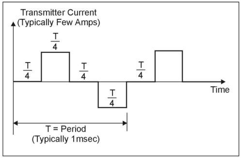
Figure 1. Transmitter current wave form.
A typical TDEM resistivity sounding survey configuration is shown in figure 2, where it is seen that the transmitter is connected to a square (usually single turn) loop of wire laid on the ground. The side length of the loop is approximately equal to the desired depth of exploration, except that for shallow depths (less than 40 m), the length can be as small as 5 to 10 m in relatively resistive ground. A multi-turn receiver coil, located at the center of the transmitter loop, is connected to the receiver through a short length of cable.
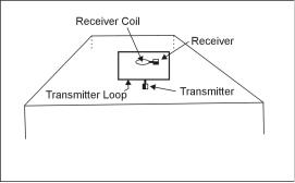
Figure 2. Central loop sounding configuration.
The principles of TDEM resistivity sounding are relatively easily understood. The process of abruptly reducing the transmitter current to zero induces, in accord with Faraday's law, a short-duration voltage pulse in the ground, which causes a loop of current to flow in the immediate vicinity of the transmitter wire, as shown in figure 3. In fact, immediately after transmitter current is turned off, the current loop can be thought of as an image in the ground of the transmitter loop. However, because of finite ground resistivity, the amplitude of the current starts to decay immediately. This decaying current similarly induces a voltage pulse that causes more current to flow, but now at a larger distance from the transmitter loop, and also at greater depth, as shown in figure 3. This deeper current flow also decays due to finite resistivity of the ground, inducing even deeper current flow and so on. The amplitude of the current flow as a function of time is measured by measuring its decaying magnetic field using a small multi-turn receiver coil usually located at the center of the transmitter loop. From the above, it is evident that, by making measurement of the voltage out of the receiver coil at successively later times, measurement is made of the current flow and thus also of the electrical resistivity of the earth at successively greater depths. This process forms the basis of central loop resistivity sounding in the time domain.
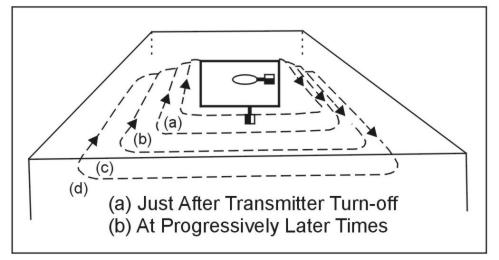
Figure 3. Transient current flow in the ground.
The output voltage of the receiver coil is shown schematically (along with the transmitter current) in figure 4. To accurately measure the decay characteristics of this voltage, the receiver contains 20 narrow time gates (indicated in figure 5), each opening sequentially to measure (and record) the amplitude of the decaying voltage at 20 successive times. Note that to minimize distortion in measurement of the transient voltage, the early time gates, which are located where the transient voltage is changing rapidly with time, are very narrow, whereas the later gates, situated where the transient is varying more slowly, are much broader. This technique is desirable since wider gates enhance the signal-to-noise ratio, which becomes smaller as the amplitude of the transient decays at later times. It will be noted from figure 4 that there are four receiver voltage transients generated during each complete period (one positive pulse plus one negative pulse) of transmitter current flow. However, measurement is made only of those two transients that occur when the transmitter current has just been shut off, since in this case, accuracy of the measurement is not affected by small errors in location of the receiver coil. This feature offers a very significant advantage over FDEM measurements, which are generally very sensitive to variations in the transmitter coil/receiver coil spacing since the FDEM receiver measures while the transmitter current is flowing. Finally, particularly for shallower sounding, where it is not necessary to measure the transient characteristics out to very late times, the period is typically of the order of 1 msec or less, which means that in a total measurement time of a few seconds, measurement can be made and stacked on several thousand transient responses. This is important since the transient response from one pulse is exceedingly small, and it is necessary to improve the signal-to-noise ratio by adding the responses from a large number of pulses.
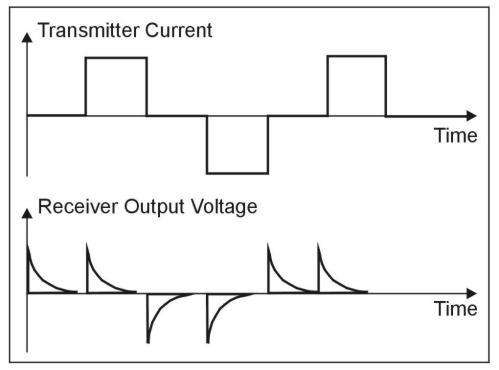
Figure 4. Receiver output wave form.
Apparent Resistivity In TDEM Soundings
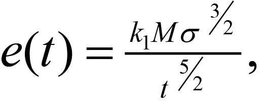
Figure 5 shows, schematically, a linear plot of typical transient response from the earth. It is useful to examine this response when plotted logarithmically against the logarithm of time, particularly if the earth is homogeneous (i.e. the resistivity does not vary with either lateral distance or depth). Such a plot is shown in figure 303, which suggests that the response can be divided into an early stage (where the response is constant with time), an intermediate stage (response shape continually varying with time), and a late stage (response is now a straight line on the log-log plot). The response is generally a mathematically complex function of conductivity and time; however, during the late stage, the mathematics simplifies considerably, and it can be shown that during this time the response varies quite simply with time and conductivity as
 (1)
(1)
where
e(t)= output voltage from a single-turn receiver coil of area 1 m2
k1 = a constant
M = product of Tx current x area (a-m2)
σ = terrain conductivity (siemens/m = S/m = 1/Ωm)
t = time (s)
Unlike the case for conventional resistivity measurement, where the measured voltage varies linearly with terrain resistivity, for TDEM, the measured voltage e(t) varies as σ3/2, so it is intrinsically more sensitive to small variations in the conductivity than conventional resistivity. Note that during the late stage, the measured voltage is decaying at the rate t-5/2, which is very rapidly with time. Eventually the signal disappears into the system noise, and further measurement is impossible. This is the maximum depth of exploration for the particular system.
Figure 5. Receiver gate locations.
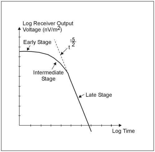
Figure 6. Log plot-receiver output voltage versus time (one transient).
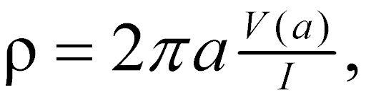
With conventional DC resistivity methods, for example the commonly used Wenner array, the measured voltage over a uniform earth can be shown to be
![]() (2a)
(2a)
where
a = interelectrode spacing (m)
ρ = terrain resistivity (Ωm)
I = current into the outer electrodes
V(a) = voltage measured across the inner electrodes for the specific value of a
In order to obtain the resistivity of the ground, equation 75a is rearranged (inverted) to give equation 75b:
 (2b)
(2b)
If ground resistivity is uniform as the interelectrode spacing (a) is increased, the measured voltage increases directly with a so that the right-hand side of equation 2b stays constant, and the equation gives the true resistivity. Suppose now that the ground is horizontally layered (i.e., that the resistivity varies with depth); for example, it might consist of an upper layer of thickness h and resistivity ρ1, overlying a more resistive basement of resistivity ρ2 > ρ1, (this is called a two-layered earth). At very short interelectrode spacing (a<<h), virtually no current penetrates into the more resistive basement, and resistivity calculation from equation 2b will give the value ρ1. As interelectrode spacing is increased, the current (I) is forced to flow to greater and greater depths. Suppose that, at large values of a (a>>h), the effect of the near-surface material of resistivity ρ1 will be negligible, and resistivity calculated from equation 2b will give the value ρ2, which is indeed what happens. At intermediate values of a (a. h), the resistivity given by equation 2b will lie somewhere between ρ1 and ρ2.
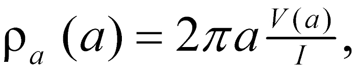
Equation 2b is, in the general case, used to define an apparent resistivity ρa(a), which is a function of a. The variation of a ρa(a) with a
 (3)
(3)
is descriptive of the variation of resistivity with depth. The behavior of the apparent resistivity ρa(a) for a Wenner array for the two-layered earth above is shown schematically in figure 7. It is clear that in conventional resistivity sounding, to increase the depth of exploration, the interelectrode spacing must be increased. In the case of TDEM soundings, on the other hand, it was observed earlier that as time increased, the depth to the current loops increased, and this phenomenon is used to perform the sounding of resistivity with depth. Thus, in analogy with equation 3, equation 4 is inverted to read (since ρ = 1/σ)
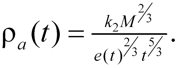 (4)
(4)
Suppose once again that terrain resistivity does not vary with depth (i.e. a uniform half-space) and is of resistivity ρ1. For this case, a plot of ρa(t) against time would be as shown in figure 8. Note that at late time the apparent resistivity ρa(t) is equal to ρ1, but at early time ρa(t) is much larger than ρ1. The reason for this is that the definition of apparent resistivity is based (as seen from figure 6) on the time behavior of the receiver coil output voltage at late time when it decays as t-5/2. At earlier and intermediate time, figure 6 shows that the receiver voltage is too low (the dashed line indicates the voltage given by the late stage approximation) and thus, from equation 4, the apparent resistivity will be too high. For this reason, there will always be, as shown on figure 8, a "descending branch" at early time where the apparent resistivity is higher than the half-space resistivity (or, as will be seen later, is higher than the upper layer resistivity in a horizontally layered earth). This is not a problem, but it is an artifact of which we must be aware.
If we let the earth be two-layered of upper layer resistivity ρ1, and thickness h, and basement resistivity ρ2 (>ρ1), at early time when the currents are entirely in the upper layer of resistivity ρ1 the decay curve will look like that of figure 6, and the apparent resistivity curve will look like figure 7. However, later on the currents will lie in both layers, and at much later time, they will be located entirely in the basement, of resistivity ρ2. Since ρ2>ρ1, equation 4 shows that, as indicated in figure 9a, the measured voltage will now be less than it should have been for the homogeneous half-space of resistivity ρ1. The effect on the apparent resistivity curve is shown in figure 10a. Since at late times all the currents are in the basement, the apparent resistivity ρa(t) becomes equal to ρ2, completely in analogy for figure 7 for conventional resistivity measurements. In the event that ρ2<ρ1, the inverse behavior is also as expected, i.e., at late times the measured voltage response, shown in figure 9b, is greater than that from a homogeneous half-space of resistivity ρ1, and the apparent resistivity curve correspondingly becomes that of figure 10b, becoming equal to the new value of ρ2 at late time. Note that for the case of a (relatively) conductive basement, there is a region of intermediate time (shown as t*), where the voltage response temporarily falls before continuing on to adopt the value appropriate to ρ2. This behavior, which is a acteristic of TDEM, is again not a problem, as long as it is recognized. The resultant influence of the anomalous behavior on the apparent resistivity is also shown on figure 10b at t*.
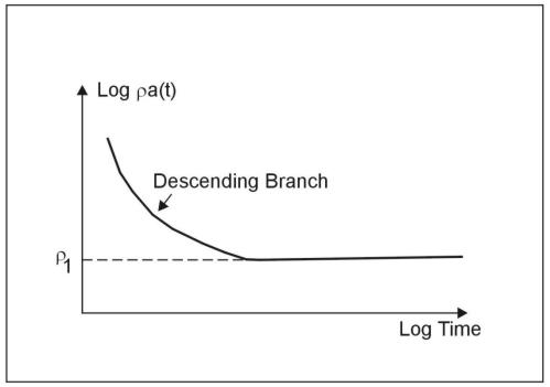
Figure 7. Wenner array: apparent resistivity, two layer curve
Figure 8. Time Domain Electromagnetic (TDEM): apparent resistivity, homogeneous half space.
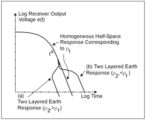
Figure 9. Time Domain Electromagnetic (TDEM): receiver output voltage, two layer earth.
To summarize, except for the early-time descending branch and the intermediate-time anomalous region described above, the sounding behavior of TDEM is analogous to that of conventional DC resistivity if the passage of time is allowed to achieve the increasing depth of exploration rather than increasing interelectrode spacing.
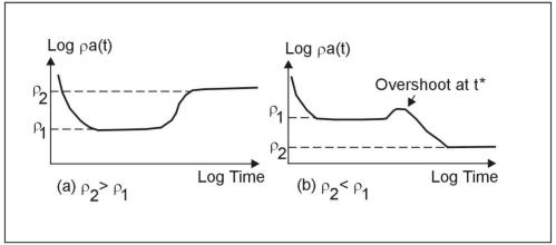
Figure 10. Time Domain Electromagnetic (TDEM): apparent resistivity, two layered earth.
Curves of apparent resistivity such as figure 10 tend to disguise the fact, that, at very late times, there is simply no signal, as is evident from figure 9. In fact, in the TDEM central loop sounding method, it is unusual to see, in practical data, the curve of apparent resistivity actually asymptote to the basement resistivity due to loss of measurable signal. Fortunately, both theoretically and in practice, the information about the behavior of the apparent resistivity curve at early time and in the transition region is generally sufficient to allow the interpretation to determine relatively accurately the resistivity of the basement without use of the full resistivity-sounding curve.
Data Acquisition
A common survey configuration consists of a square single turn loop with a horizontal receiver coil located at the center. Data from a resistivity sounding consist of a series of values of receiver output voltage at each of a succession of gate times. These gates are located in time typically from a few microseconds up to tens or even hundreds of milliseconds after the transmitter current has been turned off, depending on the desired depth of exploration. The receiver coil measures the time rate of change of the magnetic field e(t)2=dB/dt, as a function of time during the transient. Properly calibrated, the units of e(t) are V/m2 of receiver coil area; however, since the measured signals are extremely small, it is common to use nV/m2, and measured decays typically range from many thousands of nV/m2 at early times to less than 0.1 nV/m2 at late times. Modern receivers are calibrated in nV/m2 or V/m2. To check the calibration, a "Q-coil," which is a small short-circuited multi-turn coil laid on the ground at an accurate distance from the receiver coil, is often used so as to provide a transient signal of known amplitude.
The two main questions in carrying out a resistivity sounding are (a) how large should the side lengths of the (usually single-turn) transmitter be, and (b) how much current should the loop carry? Both questions are easily answered by using one of the commercially available forward layered-earth computer modeling programs. A reasonable guess as to the possible geoelectric section (i.e., the number of layers, and the resistivity and thickness of each) is made. These data are then fed into the program, along with the proposed loop size and current, and the transient voltage is calculated as a function of time. For example, assume that it is suspected that a clay aquitard may exist at a depth of 20 m in an otherwise clay-free sand. Resistivity of the sand might be 100 Ωm, and that of the clay layer 15 Ωm. Desired information includes the minimum thickness of the clay layer that is detectable, and the accuracy with which this thickness can be measured. The depth of exploration is of the order of the loop edge size, so 10 m by 10 m represents a reasonable guess for model calculation, along with a loop current of 3 A, which is acteristic of a low-power, shallow-depth transmitter. Before doing the calculations, one feature regarding the use of small (i.e., less than 60 m by 60 m) transmitter loops for shallow sounding should be noted. In these small loops, the inducing primary magnetic field at the center of the loop is very high, and the presence of any metal, such as the receiver box, or indeed the shielding on the receiver coil itself, can cause sufficient transient response to seriously distort the measured signal from the ground. This effect is greatly reduced by placing the receiver coil (and receiver) a distance of about 10 m outside the nearest transmitter edge. As shown later, the consequence of this on the data is relatively small.
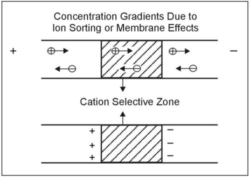
Figure 11. Nometallic induced Polarization agent. (Seigel 1970); copyright permission granted by Geological Survey of Canada)
The first task is to attempt to resolve the difference between, for example, a clay layer 0 m thick (no clay) and 1 m thick. Results of the forward layered-earth calculation, shown in figure 11, indicate that the apparent resistivity curves from these two cases are well separated (difference in calculated apparent resistivity is about 10%) over the time range from about 8 μs to 100 μs, as would be expected from the relatively shallow depths. Note that to use this early time information, a receiver is required that has many narrow early time gates in order to resolve the curve, and also has a wide bandwidth so as not to distort the early portions of the transient decay. Note from the figure that resolving thicknesses from 1 to 4 m and greater will present no problem.
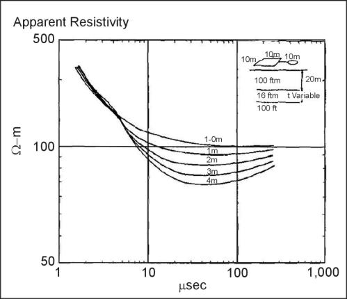
Figure 12. Forward layered-earth calculations
Having ascertained that the physics of TDEM sounding will allow detection of this thin layer, the next test is to make sure that the 10‑ by 10‑m transmitter running at 3 A will provide sufficient signal-to-noise over the time range of interest (8 to 100 μs). The same forward layered-earth calculation also outputs the actual measured voltages that would be measured from the receiver coil. These are listed (for the case of thickness of 0 m, which will produce the lowest voltage at late times) in Seismic Methods Table 1. Focus attention on the first column (which gives the time, in seconds) and the third column (which gives the receiver output as a function of time, in V/m2). The typical system noise level (almost invariably caused by external noise sources) for gates around 100 to 1,000 μs is about 0.5 nV/m2, or 5 x 10⁻¹⁰V/m2. From columns 1 and 3 see that, for the model chosen, the signal falls to 5 x 10⁻¹⁰V/m2 at a time of about 630 μs and is much greater than this for the early times when the apparent resistivity curves are well-resolved, so it is learned that the 10‑ by 10‑m transmitter at 3 A is entirely adequate. In fact, if a 5‑ by 5‑m transmitter was used, the dipole moment (product of transmitter current and area) would fall by 4, as would the measured signals, and the signal-to-noise ratio would still be excellent over the time range of interest. Thus assured, assuming that the model realistically represents the actual conditions of resistivity, the procedure will be able to detect the thin clay layer. Before proceeding with the actual measurement, it would be wise to vary some of the model parameters, such as the matrixand clay resistivities, to see under what other conditions the clay will be detectable. The importance of carrying out such calculations cannot be overstated. The theory of TDEM resistivity sounding is well understood, and the value of such modeling, which is inexpensive and fast, is very high.
It was stated above that offsetting the receiver coil from the center of the transmitter loop would not greatly affect the shape of the apparent resistivity curves. The reason for this is that the vertical magnetic field arising from a large loop of current (such as that shown in the ground at late time in figure 3) changes very slowly in moving around the loop center. Thus, at late time, when the current loop radius is significantly larger than the transmitter loop radius, it would be expected that moving the receiver from the center of the transmitter loop to outside the loop would not produce a large difference, whereas at earlier times, when the current loop radius is approximately the same as the transmitter radius, such offset will have a larger effect. This behavior is illustrated in figure 13, which shows the apparent resistivity curves for the receiver at the center and offset by 15 m from the center of the 10‑ by 10‑m transmitter loop. At late time, the curves are virtually identical.
One of the big advantages of TDEM geoelectric sounding over conventional DC sounding is that for TDEM, the overall width of the measuring array is usually much less than the depth of exploration, whereas for conventional DC sounding, the array dimension is typically (Wenner array) of the order of three times the exploration depth. Thus, in the usual event that the terrain resistivity is varying laterally, TDEM sounding will generally indicate those variations much more accurately. If the variations are very closely spaced, one might even take measurements at a station spacing of every transmitter loop length. It should be noted that most of the time spent doing a sounding (especially deeper ones where the transmitter loop is large) is utilized in laying out the transmitter loop. In this case, it can be much more efficient to have one or even two groups laying out loops in advance of the survey party, who then follow along with the actual transmitter, receiver, and receiver coil to make the sounding in a matter of minutes, again very favorable compared with DC sounding. A further advantage of TDEM geoelectric sounding is that, if a geoelectric interface is not horizontal, but is dipping, the TDEM still gives a reasonably accurate average depth to the interface. Similarly, TDEM sounding is much less sensitive (especially at later times) to varying surface topography.
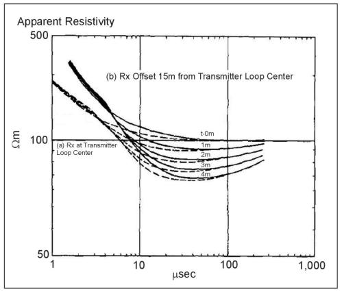
Figure 13. Forward layered earth calculations, a) central loop sounding, b) offset sounding.
It was explained above that, particularly at later times, the shape of the apparent resistivity curve is relatively insensitive to the location of the receiver coil. This feature is rather useful when the ground might be sufficiently inhomogeneous to invalidate a sounding (in the worst case, for example, due to a buried metallic pipe). In this case, a useful and quick procedure is to take several measurements at different receiver locations, as shown in figure 14. Curve 5 is obviously anomalous, and must be rejected. Curves 1-4 can all be used in the inversion process, which handles both central and offset receiver coils. Another useful way to ensure, especially for deep soundings, that the measurement is free from errors caused by lateral inhomogeneities (perhaps a nearby fault structure) is to use a three- component receiver coil, which measures, in addition to the usual vertical component of the decaying magnetic field, both horizontal components. When the ground is uniform or horizontally layered, the two horizontal components are both essentially equal to zero, as long as the measurement is made near the transmitter loop center (which is why the technique is particularly relative to deep sounding). Departures from zero are a sure indication of lateral inhomogeneities that might invalidate the sounding.
Most receivers, particularly those designed for shallower sounding, have an adjustable base frequency to permit changing the length of the measurement time. With reference to figures 1 and 4, changing the base frequency fb will change the period T (T=1/fb), and thus the measurement duration T/4. For transients that decay quickly, such as shallow sounding, the measurement period, which should be of the order of duration of the transient, should be short, and thus the base frequency high. This has the advantage that, for a given total integration time of, say 5 s, more transient responses will be stacked, to improve the signal-to-noise ratio and allow the use of smaller, more mobile, transmitter loops, increasing survey speed. On the other hand, for deep sounding, where the response must be measured out to very long time, it is clear that the measurement period must be greatly extended so that the transient response does not run on to the next primary field cycle or indeed the next transient response, and thus the base frequency must be significantly reduced. The signal-to-noise ratio will deteriorate due to fewer transients being stacked, and must be increased by either using a larger transmitter loop and transmitter current (to increase the transmitter dipole) and/or integrating the data for a longer stacking time, perhaps for 30 s or even a minute. It should be noted that should such run-on occur because too high a base frequency was employed, it can still be corrected for in modern data inversion programs; however, in extreme cases, accuracy and resolution of the inversion will start to deteriorate.
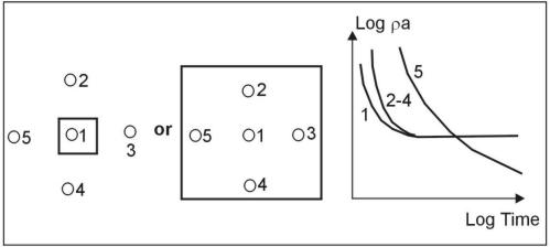
Figure 14. Offset Rx locations to check lateral homogeneity; position 5 is near lateral inhomogeneity.
In figure 4 and in this discussion, it was assumed that the transmitter current is turned off instantaneously. To actually accomplish this with a large loop of transmitter wire is impossible, and modern transmitters shut the current down using a very fast linear ramp. The duration of this ramp is maintained as short as possible (it can be shown to have an effect similar to that of broadening the measurement gate widths) particularly for shallow sounding where the transient decays very rapidly at early times. The duration of the transmitter turn-off ramp (which can also be included in modern inversion programs) is usually controlled by transmitter loop size and/or loop current.
Sources of Noise
Noise sources for TDEM soundings can be divided into four categories:
a) Circuit noise (usually so low in modern receivers as to rarely cause a problem).
b) Radiated and induced noise.
c) Presence of nearby metallic structures.
d) Soil electrochemical effects (induced polarization).
Radiated noise consists of signals generated by radio and radar transmitters and also from thunderstorm lightning activity. The first two are not usually a problem; however, on summer days when there is extensive local thunderstorm activity, the electrical noise from lightning strikes (similar to the noise heard on AM car radios) can cause problems, and it may be necessary to increase the integration (stacking) time or, in severe cases, to discontinue the survey until the storms have passed by or abated.
The most important source of induced noise consists of the intense magnetic fields from 50- to 60-Hz power lines. The large signals induced in the receiver from these fields (which fall off more or less linearly with distance from the power line) can overload the receiver if the receiver gain is set to be too high, and thus cause serious errors. The remedy is to reduce the receiver gain so that overload does not occur, although in some cases, this may result in less accurate measurement of the transient since the available dynamic range of the receiver is not being fully utilized. Another alternative is to move the measurement array further from the power line.
The response from metallic structures can be very large compared with the response from the ground. Interestingly, the power lines referred to above can often also be detected as metallic structures, as well as sources of induced noise. In this case, they exhibit an oscillating response (the response from all other targets, including the earth, decays monotonically to zero). Since the frequency of oscillation is unrelated to the receiver base frequency, the effect of power line structural response is to render the transient "noisy" as shown in figure 15. Since these oscillations arise from response to eddy currents actually induced in the power line by the TDEM transmitter, repeating the measurement will produce an identical response, which is one way that these oscillators are identified. Another way is to take a measurement with the transmitter turned off. If the "noise" disappears, it is a good indication that power-line response is the problem. The only remedy is to move the transmitter farther from the power line. Other metallic responses, such as those from buried metallic trash or pipes, can also present a problem, a solution for which was discussed in the previous section (multiple receiver sites, as shown in figure 14). If the response is very large, another sounding site must be selected. Application of another instrument such as a metal detector or ground conductivity meter to quickly survey the site for pipes can often prove useful.
A rather rare effect, but one which can occur, particularly in clayey soils, is that of induced polarization. Rapid termination of the transmitter current can ge up the minute electrical capacitors in the soil interfaces (induced polarization). These capacitors subsequently disge, producing current flow similar to that shown in figure 3, but in the opposite direction. The net effect is to reduce the amplitude of the transient response (thus increasing the apparent resistivity) or even, where the effect is very severe, to cause the transient response to become negative over some range of the measurement time. Since these sources of reverse current are localized near the transmitter loop, using the offset configuration usually reduces the errors caused by them to small values.
In summary, it should be noted that in TDEM soundings, the signal-to-noise ratio is usually very good over most of the time range. However, in general, the transient response is decaying extremely rapidly (of the order of t-5/2, or by a factor of about 300 for a factor of 10 increase in time). The result is that toward the end of the transient, the signal-to-noise ratio suddenly deteriorates completely, and the data become exceedingly noisy. The transient is over!
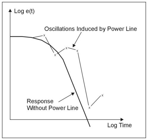
Figure 15. Oscillations induced in receiver response by power line.
Data Processing and Interpretation
In the early days of TDEM sounding, particularly in Russia where the technique was developed (Kaufman and Keller 1983), extensive use was made of numerically calculated apparent resistivity curves for a variety of layered earth geometrics. Field data would be compared with a selection of curves, from which the actual geoelectric section would be determined. More recently, the advent of relatively fast computer inversion programs allows field transient data to be automatically inverted to a layered earth geometry in a matter of minutes. An inversion program offers an additional significant advantage. All electrical sounding techniques (conventional DC, magneto-telluric, TDEM) suffer to a greater or less extent from equivalence, which basically states that, to within a given signal-to-noise ratio in the measured data, more than one specific geoelectric model will fit the measured data. This problem, which is seldom addressed in conventional DC soundings, is one of which the interpreter must be aware, and the advantage of the inversion program is that, given an estimate of the signal-to-noise ratio in the measured data, the program could calculate a selection of equivalent geoelectric sections that will also fit the measured data, immediately allowing the interpreter to decide exactly how unique his solution really is. Equivalence is a fact of life, and must be included in any interpretation.
Advantages and Limitations
The advantages of TDEM geoelectric sounding over conventional DC resistivity sounding are significant. They include the following:
1. Improved speed of operation.
2. Improved lateral resolution.
3. Improved resolution of conductive electrical equivalence.
4. No problems injecting current into a resistive surface layer.
The limitations of TDEM techniques are as follows:
1. Do not work well in very resistive material.
2. Interpretational material for TDEM on, for example, 3D structures is still under development.
3. TDEM equipment tends to be somewhat more costly due to its greater complexity.
As mentioned above, the advantages are significant, and TDEM is becoming a widely used tool for geoelectrical sounding.
Two Dimensional Imaging
As in multiple other geophysical techniques, and with the advent of computers with greater processing strengths, two-dimensional imaging using the one dimensional approaches, has become common place. By completing a series of one dimensional soundings, a two dimensional image can be generated from the resulting data. Figure 16 presents an example of a two dimensional image generated from a series of one dimensional, inverted TEM soundings, and resulting interpretation.
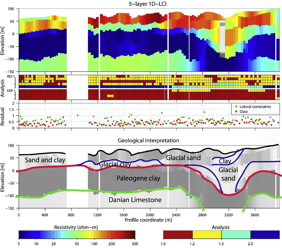
Figure 16. Two dimensional imaging results using stitched together one dimensional inversion results for a 5 layer model These images are presented for references purposes only, no endorsement of the software is intended.
The pages found under Surface Methods and Borehole Methods are substantially based on a report produced by the United States Department of Transportation:
Wightman, W. E., Jalinoos, F., Sirles, P., and Hanna, K. (2003). "Application of Geophysical Methods to Highway Related Problems." Federal Highway Administration, Central Federal Lands Highway Division, Lakewood, CO, Publication No. FHWA-IF-04-021, September 2003. http://www.cflhd.gov/resources/agm/![]()