Surface Wave Methods
Introduction
A wide variety of seismic waves propagate along the surface of the earth. They are called surface waves because their amplitude decreases exponentially with increasing depth. The Rayleigh wave is important in engineering studies because of its simplicity and because of the close relationship of its velocity to the shear-wave velocity for earth materials. As most earth materials have Poisson's ratios in the range of 0.25 to 0.48, the approximation of Rayleigh wave velocities as shear-wave velocities causes less than a 10% error. Rayleigh wave studies for engineering purposes have most often been made in the past by direct observation of the Rayleigh wave velocities. One method consists of excitation of a monochromatic wave train and the direct observation of the travel time of this wave train between two points. As the frequency is known, the wavelength is determined by dividing the velocity by the frequency.
The assumption that the depth of investigation is equal to one-half of the wavelength can be used to generate a velocity profile with depth. This last assumption is somewhat supported by surface wave theory, but more modern and comprehensive methods are available for inversion of Rayleigh-wave observations. Similar data can be obtained from impulsive sources if the recording is made at sufficient distance such that the surface wave train has separated into its separate frequency components.
Spectral Analysis of Surface Waves (SASW)
The promise, both theoretical and observational, of surface wave methods has resulted in significant applications of technology to their exploitation. The problem is twofold:
To determine, as a function of frequency, the velocity of surface waves traveling along the surface (this curve, often presented as wavelength versus phase velocity, is called a dispersion curve).
From the dispersion curve, determine an earth structure that would exhibit such dispersion. This inversion, which is ordinarily done by forward modeling, has been automated with varying degrees of success.
Basic Concept
Spectral analysis, via the Fourier transform, can convert any time-domain function into its constituent frequencies. Cross-spectral analysis yields two valuable outputs from the simultaneous spectral analysis of two time functions. One output is the phase difference between the two time functions as a function of frequency. This phase difference spectrum can be converted to a time difference (as a function of frequency) by use of the relationship:
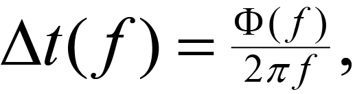 (1)
(1)
where
Δt( f )= frequency-dependent time difference,
Φ( f ) = cross-spectral phase at frequency f,
f= frequency to which the time difference applies.
If the two time functions analyzed are the seismic signals recorded at two geophones a distance d apart, then the velocity, as a function of frequency, is given by:
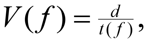 (2)
(2)
where
d = distance between geophones,
t( f )= term determined from the cross-spectral phase.
If the wavelength (λ) is required, it is given by:
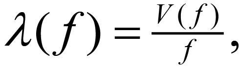 (3)
(3)
As these mathematical operations are carried at for a variety of frequencies, an extensive dispersion curve is generated. The second output of the cross-spectral analysis that is useful in this work is the coherence function. This output measures the similarity of the two inputs as a function of frequency. Normalized to lie between 0 and 1, a coherency of greater than 0.9 is often required for effective phase difference estimates. Once the dispersion curve is in hand, the calculation-intensive inversion process can proceed. Although the assumption given above of depth equal to one-half the wavelength may be adequate if relatively few data are available, the direct calculation of a sample dispersion curve from a layered model is necessary to account for the abundance of data that can be recorded by a modern seismic system. Whether or not the inversion is automated, the requirements for a good geophysical inversion should be followed, and more observations than parameters should be selected.
Calculation methods for the inversion are beyond the scope of this manual. The model used is a set of flat-lying layers made up of thicknesses and shear-wave velocities. More layers are typically used than are suspected to be present, and one useful iteration is to consolidate the model layers into a geologically consistent model and repeat the inversion for the velocities only.
The advantages of this method are:
a) High frequencies (1-300 Hz) can be used, resulting in definition of very thin layers.
b) The refraction requirement of increasing velocities with depth is not present; thus, velocities that decrease with depth are detectable.
By using both of these advantages, this method has been used to investigate pavement substrate strength. An example of typical data obtained by an SASW experiment is shown in figure 1. The scatter of these data is smaller than typical SASW data. Models obtained by two different inversion schemes are shown in figure 2 along with some crosshole data for comparison. Note that the agreement is excellent above 20 m of depth.
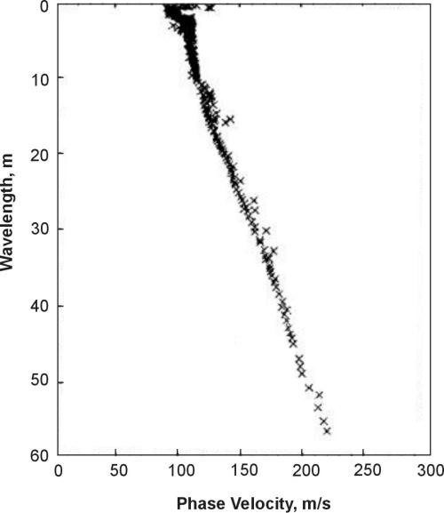
Figure 1. Typical Spectral Analysis of Surface Waves data.
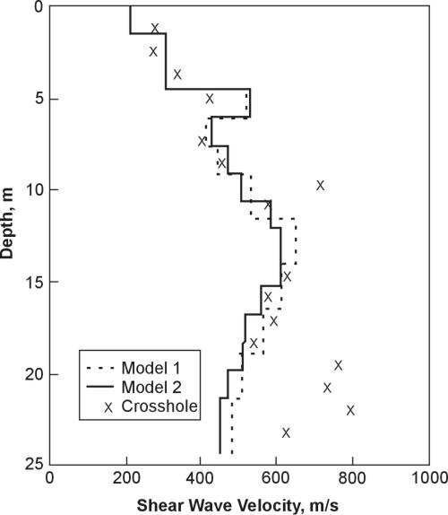
Figure 2. Inversion results of typical Spectral Analysis of Surface Waves data.
Data Acquisition
Most crews are equipped with a two- or four-channel spectrum analyzer, which provides the cross-spectral phase and coherence information. The degree of automation of the subsequent processing varies widely from laborious manual entry of the phase velocities into an analysis program to automated acquisition and preliminary processing. The inversion process similarly can be based on forward modeling with lots of human interaction or true inversion by computer after some manual smoothing.
A typical SASW crew consists of two persons, one to operate and coordinate the source and one to monitor the quality of the results. Typical field procedures are to place two (or four) geophones or accelerometers close together and to turn on the source. The source may be any mechanical source of high-frequency energy; moving bulldozers, dirt whackers, hammer blows, and vibrators have been used. Some discretion is advised as the source must operate for long periods of time, and the physics of what is happening are important. Rayleigh waves have predominantly vertical motion; thus, a source whose impedance is matched to the soil and whose energy is concentrated in the direction and frequency band of interest will be more successful.
Phase velocities are determined for waves with wavelength from 0.5 to 3 times the distance between the geophones. Then the phones are moved apart, usually increasing the separation by a factor of two. Thus, overlapping data are acquired, and the validity of the process is checked. This process continues until the wavelength being measured is equal to the required depth of investigation. Then the apparatus is moved to the next station where a sounding is required. After processing, a vertical profile of the shear-wave velocities is produced.
Advantages and Limitations
1. The assumption of plane layers from the source to the recording point may not be accurate.
2. Higher modes of the Rayleigh wave may be recorded. The usual processing assumption is that the fundamental mode has been measured.
3. Spreading the geophones across a lateral inhomogeneity will produce complications beyond the scope of the method.
4. Very high frequencies may be difficult to generate and record.
Common-Offset Rayleigh Wave Method
This method is also called Common-Offset Surface Waves. The method is quite effective at mapping inhomogeneities in the near surface, although it is not a frequently used method. The field techniques are easy to apply, and compared to other seismic methods, it is a rapid technique.
This method uses Rayleigh waves to detect fracture zones and associated voids. Rayleigh waves, also known as surface waves, have a particle motion that is counterclockwise with respect to the direction of travel. Figure 3 illustrates the particle motion for Rayleigh waves traveling in the positive X direction. In addition, the particle displacement is greatest at the ground surface, near the Rayleigh wave source, and decreases with depth. Three shot points are shown, labeled A, B, and C. The particle motion and displacement are shown for five depths under each shot point. For shot B, over the void, no Rayleigh waves are transmitted through the water/air filled void. This affects the measured Rayleigh wave recorded by the geophones over the void. Four parameters are usually observed. The first is an increase in the travel time of the Rayleigh wave as the fracture zone above the void is crossed. The second parameter is a decrease in the amplitude of the Rayleigh wave. The third parameter is reverberations (sometimes called ringing) as the void is crossed. The fourth parameter is a shift in the peak frequency toward lower frequencies. This is caused by trapped waves, similar to a tube wave in a borehole. The effective depth of penetration is approximately one-third to one-half of the wavelength of the Rayleigh wave.
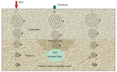
Figure 3. Rayleigh wave particle motion and displacement.
Rayleigh waves are created by any impact source. For shallow investigations, a hammer is all that is needed. Data are recorded using one geophone and one shot point. The distance between the shot and geophone depends on the depth of investigation and is usually about twice the expected target depth. Data are recorded at regular intervals across the traverse while maintaining the same shot geophone separation. The interval between stations depends on the expected size of the void/fracture zone and the desired resolution. Generally, in order to clearly see the void/fracture zone, it is desirable to have several stations that cross the area of interest. Figure 3 presents data from a common offset Rayleigh wave survey over a void/fracture zone in an alluvial basin. The geophone traces are drawn horizontally with the vertical axis being distance (shot stations).
The data may be filtered to highlight the Rayleigh wave frequencies and is then plotted as shown on figure 4. Because the peak frequency of the seismic signal decreases over a void/fracture zone, a spectral analysis of the traces can assist in the interpretation of the data by highlighting the traces with lower frequencies. The data shown in figure 4 illustrate many of the features expected over a void/fracture zone. The travel time to the first arrival of the Rayleigh wave is greater across the void/fracture and is wider than the actual fractured zone. The amplitudes of the Rayleigh waves decrease as the zone is crossed. In addition, the wavelength of the signals over the fracture/void is longer than those over unfractured rock, showing that the high frequencies have been attenuated. Since the records are not long enough, the ringing effect is not presented in these data.
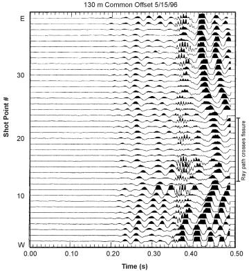
Figure 4. Data from a Rayleigh wave survey over a void/fracture zone.
Rayleigh waves are influenced by the shear strength of the rocks as well as fractures and voids, and changes in shear strength can cause anomalies similar to those obtained over these features. The depth of penetration and target resolution are influenced by the wavelengths generated by the seismic source. Since longer wavelengths, which have lower resolution, are needed to investigate to greater depths, fractures and voids at depth need to be increasingly larger in order to be observed. However, this method is faster and less costly than most other seismic methods.
The pages found under Surface Methods and Borehole Methods are substantially based on a report produced by the United States Department of Transportation:
Wightman, W. E., Jalinoos, F., Sirles, P., and Hanna, K. (2003). "Application of Geophysical Methods to Highway Related Problems." Federal Highway Administration, Central Federal Lands Highway Division, Lakewood, CO, Publication No. FHWA-IF-04-021, September 2003. http://www.cflhd.gov/resources/agm/![]()