Resistivity Methods
Introduction
Surface electrical resistivity surveying is based on the principle that the distribution of electrical potential in the ground around a current-carrying electrode depends on the electrical resistivities and distribution of the surrounding soils and rocks. The usual practice in the field is to apply an electrical direct current (DC) between two electrodes implanted in the ground and to measure the difference of potential between two additional electrodes that do not carry current. Usually, the potential electrodes are in line between the current electrodes, but in principle, they can be located anywhere. The current used is either direct current, commutated direct current (i.e., a square-wave alternating current), or AC of low frequency (typically about 20 Hz). All analysis and interpretation are done on the basis of direct currents. The distribution of potential can be related theoretically to ground resistivities and their distribution for some simple cases, notably, the case of a horizontally stratified ground and the case of homogeneous masses separated by vertical planes (e.g., a vertical fault with a large throw or a vertical dike). For other kinds of resistivity distributions, interpretation is usually done by qualitative comparison of observed response with that of idealized hypothetical models or on the basis of empirical methods.
Mineral grains comprised of soils and rocks are essentially nonconductive, except in some exotic materials such as metallic ores, so the resistivity of soils and rocks is governed primarily by the amount of pore water, its resistivity, and the arrangement of the pores. To the extent that differences of lithology are accompanied by differences of resistivity, resistivity surveys can be useful in detecting bodies of anomalous materials or in estimating the depths of bedrock surfaces. In coarse, granular soils, the groundwater surface is generally marked by an abrupt change in water saturation and thus by a change of resistivity. In fine-grained soils, however, there may be no such resistivity change coinciding with a piezometric surface. Generally, since the resistivity of a soil or rock is controlled primarily by the pore water conditions, there are wide ranges in resistivity for any particular soil or rock type, and resistivity values cannot be directly interpreted in terms of soil type or lithology. Commonly, however, zones of distinctive resistivity can be associated with specific soil or rock units on the basis of local field or drill hole information, and resistivity surveys can be used profitably to extend field investigations into areas with very limited or nonexistent data. Also, resistivity surveys may be used as a reconnaissance method, to detect anomalies that can be further investigated by complementary geophysical methods and/or drill holes.
The electrical resistivity method has some inherent limitations that affect the resolution and accuracy that may be expected from it. Like all methods using measurements of a potential field, the value of a measurement obtained at any location represents a weighted average of the effects produced over a large volume of material, with the nearby portions contributing most heavily. This tends to produce smooth curves, which do not lend themselves to high resolution for interpretations. Another feature common to all potential field geophysical methods is that a particular distribution of potential at the ground surface does not generally have a unique interpretation. Although these limitations should be recognized, the non-uniqueness or ambiguity of the resistivity method is scarcely less than with the other geophysical methods. For these reasons, it is always advisable to use several complementary geophysical methods in an integrated exploration program rather than relying on a single exploration method.
Theory
Data from resistivity surveys are customarily presented and interpreted in the form of values of apparent resistivity ρa. Apparent resistivity is defined as the resistivity of an electrically homogeneous and isotropic half-space that would yield the measured relationship between the applied current and the potential difference for a particular arrangement and spacing of electrodes. An equation giving the apparent resistivity in terms of applied current, distribution of potential, and arrangement of electrodes can be arrived at through an examination of the potential distribution due to a single current electrode. The effect of an electrode pair (or any other combination) can be found by superposition. Consider a single point electrode, located on the boundary of a semi-infinite, electrically homogeneous medium, which represents a fictitious homogeneous earth. If the electrode carries a current I, measured in amperes (a), the potential at any point in the medium or on the boundary is given by:
 (1)
(1)
where
U = potential, in V,
ρ = resistivity of the medium,
r = distance from the electrode.
The mathematical demonstration for the derivation of the equation may be found in textbooks on geophysics, such as Keller and Frischknecht (1966).
For an electrode pair with current I at electrode A, and -I at electrode B (figure 1), the potential at a point is given by the algebraic sum of the individual contributions:
 (2)
(2)
where
rA and rB = distances from the point to electrodes A and B
Figure 1 illustrates the electric field around the two electrodes in terms of equipotentials and current lines. The equipotentials represent imagery shells, or bowls, surrounding the current electrodes, and on any one of which the electrical potential is everywhere equal. The current lines represent a sampling of the infinitely many paths followed by the current, paths that are defined by the condition that they must be everywhere normal to the equipotential surfaces.
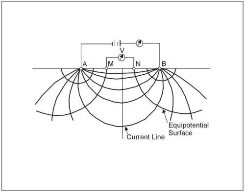
Figure 1. Equipotentials and current lines for a pair of current electrodes A and B on a homogeneous half-space.
In addition to current electrodes A and B, figure 1 shows a pair of electrodes M and N, which carry no current, but between which the potential difference V may be measured. Following the previous equation, the potential difference V may be written
 (3)
(3)
where
UM and UN = potentials at M and N,
AM = distance between electrodes A and M, etc.
These distances are always the actual distances between the respective electrodes, whether or not they lie on a line. The quantity inside the brackets is a function only of the various electrode spacings. The quantity is denoted 1/K, which allows rewriting the equation as:
 (4)
(4)
where
K = array geometric factor.
Equation 58 can be solved for ρ to obtain:
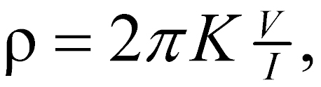 (5)
(5)
The resistivity of the medium can be found from measured values of V, I, and K, the geometric factor. K is a function only of the geometry of the electrode arrangement.
Apparent Resistivity
Wherever these measurements are made over a real heterogeneous earth, as distinguished from the fictitious homogeneous half-space, the symbol ρ is replaced by ρa for apparent resistivity. The resistivity surveying problem is, reduced to its essence, the use of apparent resistivity values from field observations at various locations and with various electrode configurations to estimate the true resistivities of the several earth materials present at a site and to locate their boundaries spatially below the surface of the site.
An electrode array with constant spacing is used to investigate lateral changes in apparent resistivity reflecting lateral geologic variability or localized anomalous features. To investigate changes in resistivity with depth, the size of the electrode array is varied. The apparent resistivity is affected by material at increasingly greater depths (hence larger volume) as the electrode spacing is increased. Because of this effect, a plot of apparent resistivity against electrode spacing can be used to indicate vertical variations in resistivity.
The types of electrode arrays that are most commonly used (Schlumberger, Wenner, and dipole-dipole) are illustrated in figure 2. There are other electrode configurations that are used experimentally or for non-geotechnical problems or are not in wide popularity today. Some of these include the Lee, half-Schlumberger, polar dipole, bipole dipole, and gradient arrays. In any case, the geometric factor for any four-electrode system can be found from equation 3 and can be developed for more complicated systems by using the rule illustrated by equation 2. It can also be seen from equation 58 that the current and potential electrodes can be interchanged without affecting the results; this property is called reciprocity.
Schlumberger Array
For this array (figure 2a), in the limit as a approaches zero, the quantity V/a approaches the value of the potential gradient at the midpoint of the array. In practice, the sensitivity of the instruments limits the ratio of s to a and usually keeps it within the limits of about 3 to 30. Therefore, it is typical practice to use a finite electrode spacing and equation 2 to compute the geometric factor (Keller and Frischknecht, 1966). The apparent resistivity (r) is:
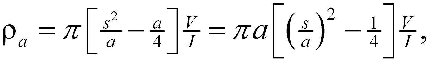 (6)
(6)
In usual field operations, the inner (potential) electrodes remain fixed, while the outer (current) electrodes are adjusted to vary the distance s. The spacing a is adjusted when it is needed because of decreasing sensitivity of measurement. The spacing a must never be larger than 0.4s or the potential gradient assumption is no longer valid. Also, the a spacing may sometimes be adjusted with s held constant in order to detect the presence of local inhomogeneities or lateral changes in the neighborhood of the potential electrodes.
Wenner Array
This array (figure 2b) consists of four electrodes in line, separated by equal intervals, denoted a. Applying equation 2, the user will find that the geometric factor K is equal to a , so the apparent resistivity is given by:
(7)
Although the Schlumberger array has always been the favored array in Europe, until recently, the Wenner array was used more extensively than the Schlumberger array in the United States. In a survey with varying electrode spacing, field operations with the Schlumberger array are faster, because all four electrodes of the Wenner array are moved between successive observations, but with the Schlumberger array, only the outer ones need to be moved. The Schlumberger array also is said to be superior in distinguishing lateral from vertical variations in resistivity. On the other hand, the Wenner array demands less instrument sensitivity, and reduction of data is marginally easier.
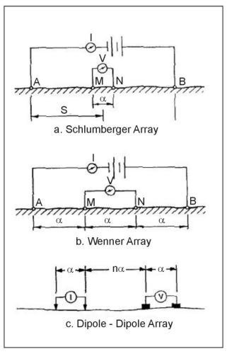
Figure 2. Electrode array configurations for resistivity measurements.
Dipole-dipole Array
The dipole-dipole array (figure 2c) is one member of a family of arrays using dipoles (closely spaced electrode pairs) to measure the curvature of the potential field. If the separation between both pairs of electrodes is the same a, and the separation between the centers of the dipoles is restricted to a(n+1), the apparent resistivity is given by:
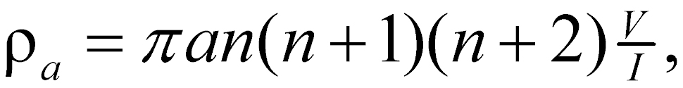 (8)
(8)
This array is especially useful for measuring lateral resistivity changes and has been increasingly used in geotechnical applications.
Depth of Investigation
To illustrate the major features of the relationship between apparent resistivity and electrode spacing, figure 3 shows a hypothetical earth model and some hypothetical apparent resistivity curves. The earth model has a surface layer of resistivity ρ1 and a basement layer of resistivity ρn that extends downward to infinity (figure 3a). There may be intermediate layers of arbitrary thicknesses and resistivities. The electrode spacing may be either the Wenner spacing a or the Schlumberger spacing a; curves of apparent resistivity versus spacing will have the same general shape for both arrays, although they will not generally coincide.
For small electrode spacings, the apparent resistivity is close to the surface layer resistivity, whereas at large electrode spacings, it approaches the resistivity of the basement layer. Every apparent resistivity curve thus has two asymptotes, the horizontal lines ρa = ρ1 and ρa = ρn, that it approaches at extreme values of electrode spacing. This is true whether ρn is greater than ρ1, as shown in figure 3b, or the reverse. The behavior of the curve between the regions where it approaches the asymptotes depends on the distribution of resistivities in the intermediate layers. Curve A represents a case in which there is an intermediate layer with a resistivity greater than ρn. The behavior of curve B resembles that for the two-layer case or a case where resistivities increase from the surface down to the basement. The curve might look like curve C if there were an intermediate layer with resistivity lower than ρ1. Unfortunately for the interpreter, neither the maximum of curve A nor the minimum of curve C reach the true resistivity values for the intermediate layers, though they may be close if the layers are very thick.
There is no simple relationship between the electrode spacing at which features of the apparent resistivity curve are located and the depths to the interfaces between layers. The depth of investigation will ALWAYS be less than the electrode spacing. Typically, a maximum electrode spacing of three or more times the depth of interest is necessary to assure that sufficient data have been obtained. The best general guide to use in the field is to plot the apparent resistivity curve (figure 2b) as the survey progresses, so that it can be judged whether the asymptotic phase of the curve has been reached.
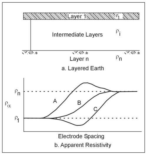
Figure 3. Asymptotic behavior of the apparent resistivity curves at very small and very large electrode spacings.
Instruments and Measurements
The theory and field methods used for resistivity surveys are based on the use of direct current, because it allows greater depth of investigation than alternating current and because it avoids the complexities caused by effects of ground inductance and capacitance and resulting frequency dependence of resistivity. However, in practice, actual direct current is infrequently used for two reasons: (1) direct current electrodes produce polarized ionization fields in the electrolytes around them, and these fields produce additional electromotive forces that cause the current and potentials in the ground to be different from those in the electrodes; and (2) natural Earth currents (telluric currents) and spontaneous potentials, which are essentially unidirectional or slowly time-varying, induce potentials in addition to those caused by the applied current. The effects of these phenomena, as well as any others that produce unidirectional components of current or potential gradients, are reduced by the use of alternating current, because the polarized ionization fields do not have sufficient time to develop in a half-cycle, and the alternating component of the response can be measured independently of any superimposed direct currents. The frequencies used are very low, typically below 20 Hz, so that the measured resistivity is essentially the same as the direct current resistivity.
In concept, a direct current (I), or an alternating current of low frequency, is applied to the current electrodes, and the current is measured with an ammeter. Independently, a potential difference V is measured across the potential electrodes, and, ideally, there should be no current flowing between the potential electrodes. This is accomplished either with a null-balancing galvanometer (old technology) or very high input impedance operational amplifiers. A few resistivity instruments have separate "sending" and "receiving" units for current and potential; but in usual practice, the potential measuring circuit is derived from the same source as the potential across the current electrodes, so that variations in the supply voltage affect both equally and do not affect the balance point.
Power is usually supplied by dry cell batteries in the smaller instruments and motor generators in the larger instruments. From 90 V up to several hundred volts may be used across the current electrodes in surveys for engineering purposes. In the battery-powered units, the current usually is small and is applied only for very short times while the potential is being measured, so battery consumption is low. Care should be taken to NEVER energize the electrodes while they are being handled, because with applied potentials of hundreds of volts, DANGEROUS AND POTENTIALLY LETHAL shocks could be caused.
Current electrodes used with alternating current (or commutated direct current) instruments commonly are stakes of bronze, copper, steel with bronze jackets, or, less desirably, steel, about 50 cm in length. They must be driven into the ground far enough to make good electrical contact. If there is difficulty because of high contact resistance between electrodes and soil, it can sometimes be alleviated by pouring salt water around the electrodes. Many resistivity instruments include an ammeter to verify that the current between the current electrodes is at an acceptable level, a desirable feature. Other instruments simply output the required potential difference to drive a selected current into the current electrodes. Typical currents in instruments used for engineering applications range from 2 mA to 500 mA. If the current is too small, the sensitivity of measurement is degraded. The problem may be corrected by improving the electrical contacts at the electrodes. However, if the problem is due to a combination of high earth resistivity and large electrode spacing, the remedy is to increase the voltage across the current electrodes. Where the ground is too hard or rocky to drive stakes, a common alternative is sheets of aluminum foil buried in shallow depressions or within small mounds of earth and wetted.
One advantage of the four-electrode method is that measurements are not sensitive to contact resistance at the potential electrodes so long as it is low enough that a measurement can be made, because observations are made with the system adjusted so that there is no current in the potential electrodes. With zero current, the actual value of contact resistance is immaterial, since it does not affect the potential. On the current electrodes also, the actual value of contact resistance does not affect the measurement, so long as it is small enough that a satisfactory current is obtained, and so long as there is no gross difference between the two electrodes. Contact resistance affects the relationship between the current and the potentials on the electrodes, but because only the measured value of current is used, the potentials on these electrodes do not figure in the theory or interpretation.
When direct current is used, special provisions must be made to eliminate the effects of electrode polarization and telluric currents. A nonpolarizing electrode is available in the form of a porous, unglazed ceramic pot, which contains a central metallic electrode, usually copper, and is filled with a liquid electrolyte that is a saturated solution of a salt of the same metal (copper sulphate is used with copper). The central electrode is connected to the instrument, and electrical contact with the ground is made through the electrolyte in the pores of the ceramic pot. This type of electrode may be advantageous for use on rock surfaces where driving rod-type electrodes is difficult. Good contact of the pot with the ground can be aided by clearing away grass and leaves beneath it, embedding it slightly in the soil, and if the ground is dry, pouring a small amount of water on the surface before placing the pot. The pots must be filled with electrolyte several hours before they are used to allow the electrolyte to penetrate the fine pores of the ceramic. The porous pot electrodes should be checked every several hours during the field day to verify the electrolyte level and the presence of the solid salt to maintain the saturated solution.
Telluric currents are naturally occurring electric fields that are widespread, some being of global scale. They are usually of small magnitude, but may be very large during solar flares or if supplemented by currents of artificial origin. Spontaneous potentials in the earth may be generated by galvanic phenomena around electrochemically active materials, such as pipes, conduits, buried scrap materials, cinders, and ore deposits. They may also occur as streaming potentials generated by groundwater movement. (Electric fields associated with groundwater movement will have the greatest amplitude where groundwater flow rates are high, such as through subsurface open-channel flow. Groundwater movement in karst areas can exhibit rapid flow through dissolved channels within the rock. Springs and subsurface flow may be the cause of telluric sources, which may obscure resistivity measurements.) Telluric currents and spontaneous potential effects can be compensated by applying a bias potential to balance the potential electrodes before energizing the current electrodes. Because telluric currents generally vary with time, frequent adjustments to the bias potential may be necessary in the course of making an observation. If the instrument lacks a provision for applying a bias potential, a less satisfactory alternative is to use a polarity-reversing switch to make readings with alternately reversed current directions in the current electrodes. The average values of V and I for the forward and reverse current directions are then used to compute the apparent resistivity.
Layout of electrodes should be done with nonconducting measuring tapes, since tapes of conducting materials, if left on the ground during measurement, can influence apparent resistivity values. Resistivity measurements can also be affected by metallic fences, rails, pipes, or other conductors, which may induce spontaneous potentials and provide short-circuit paths for the current. The effects of such linear conductors as these can be minimized, but not eliminated, by laying out the electrode array on a line perpendicular to the conductor; but in some locations, such as some urban areas, there may be so many conductive bodies in the vicinity that this cannot be done. Also, electrical noise from power lines, cables, or other sources may interfere with measurements. Because of the nearly ubiquitous noise from 60-Hz power sources in the United States, the use of 60 Hz or its harmonics in resistivity instruments is not advisable. In some cases, the quality of data affected by electrical noise can be improved by averaging values obtained from a number of observations; sometimes electrical noise comes from temporary sources, so better measurements can be obtained by waiting until conditions improve. Occasionally, ambient electrical noise and other disturbing factors at a site may make resistivity surveying infeasible. Modern resistivity instruments have capability for data averaging or stacking; this allows resistivity surveys to proceed in spite of most noisy site conditions and to improve signal-to-noise ratio for weak signals.
Data Acquisition
Resistivity surveys are made to satisfy the needs of two distinctly different kinds of interpretation problems: (1) the variation of resistivity with depth, reflecting more or less horizontal stratification of earth materials; and (2) lateral variations in resistivity that may indicate soil lenses, isolated ore bodies, faults, or cavities. For the first kind of problem, measurements of apparent resistivity are made at a single location (or around a single center point) with systematically varying electrode spacings. This procedure is sometimes called vertical electrical sounding (VES), or vertical profiling. Surveys of lateral variations may be made at spot or grid locations or along definite lines of traverse, a procedure sometimes called horizontal profiling.
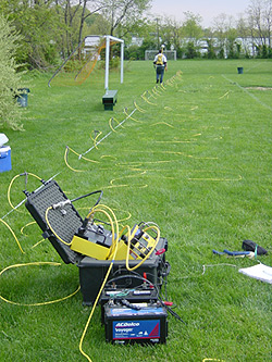
Figure 4. DC Resistivity data acquisition system deployed for site charachterization (http://water.usgs.gov/ogw/bgas/toxics/NAWC-surface.html). This image is provided for demonstration purposes, and is not intended as an endorsement for use of this product.
Vertical Electrical Sounding (VES) - 1D Imaging
Either the Schlumberger or, less effectively, the Wenner array is used for sounding, since all commonly available interpretation methods and interpretation aids for sounding are based on these two arrays. In the use of either method, the center point of the array is kept at a fixed location, while the electrode locations are varied around it. The apparent resistivity values, and layer depths interpreted from them, are referred to the center point.
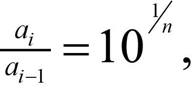
In the Wenner array, the electrodes are located at distances of a/2 and 3a/2 from the center point. The most convenient way to locate the electrode stations is to use two measuring tapes, pinned with their zero ends at the center point and extending away from the center in opposite directions. After each reading, each potential electrode is moved out by half the increment in electrode spacing, and each current electrode is moved out by 1.5 times the increment. The increment to be used depends on the interpretation methods that will be applied. In most interpretation methods, the curves are sampled at logarithmically spaced points. The ratio between successive spacings can be obtained from the relation
 (9)
(9)
where
n = number of points to be plotted in each logarithmic cycle.
For example, if six points are wanted for each cycle of the logarithmic plot, then each spacing a will be equal to 1.47 times the previous spacing. The sequence starting at 10 m would then be 10, 14.7, 21.5, 31.6, 46.4, 68.2, which, for convenience in layout and plotting, could be rounded to 10, 15, 20, 30, 45, 70. In the next cycle, the spacings would be 100, 150, 200, and so on. Six points per cycle is the minimum recommended; 10, 12, or even more per cycle may be necessary in noisy areas.
VES surveys with the Schlumberger array are also made with a fixed center point. An initial spacing s (the distance from the center of the array to either of the current electrodes) is chosen, and the current electrodes are moved outward with the potential electrodes fixed. According to Van Nostrand and Cook (1966), errors in apparent resistivity are within 2 to 3 percent if the distance between the potential electrodes does not exceed 2s/5. Potential electrode spacing is, therefore, determined by the minimum value of s. As s is increased, the sensitivity of the potential measurement decreases; therefore, at some point, if s becomes large enough, it will be necessary to increase the potential electrode spacing. The increments in s should normally be logarithmic and can be chosen in the same way as described for the Wenner array.
For either type of electrode array, minimum and maximum spacings are governed by the need to define the asymptotic phases of the apparent resistivity curve and the needed depth of investigation. Frequently, the maximum useful electrode spacing is limited by available time, site topography, or lateral variations in resistivity. For the purpose of planning the survey, a maximum electrode spacing of at least three times the depth of interest may be used, but the apparent resistivity curve should be plotted as the survey progresses in order to judge whether sufficient data have been obtained. Also, the progressive plot can be used to detect errors in readings or spurious resistivity values due to local effects. Sample field data sheets are shown in figures 4 through 6.
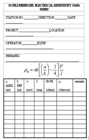
Figure 4. Example data sheet for Schlumberger vertical sounding.
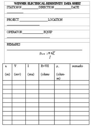
Figure 5. Example data sheet for Wenner array.
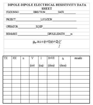
Figure 6. Example data sheet for dipole-dipole array.
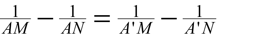
In a normal series of observations, the total resistance, R = V/I, decreases with increasing electrode spacing. Occasionally, the normal relationship may be reversed for one or a few readings. If these reversals are not a result of errors in reading, they are caused by some type of lateral or local changes in resistivity of the soil or rock. Such an effect can be caused by one current electrode being placed in a material of much higher resistivity than that around the other, for instance, in a pocket of dry gravel in contact with a boulder of highly resistive rock or close to an empty cavity. Systematic reversals might be caused by thinning of a surface conductive stratum where an underlying resistant stratum approaches the surface because it dips steeply or because of surface topography. In hilly terrains, the line of electrodes should be laid out along a contour if possible. Where beds are known to dip steeply (more than about 10 deg), the line should be laid out along the strike. Electrodes should not be placed in close proximity to boulders, so it may sometimes be necessary to displace individual electrodes away from the line. The theoretically correct method of displacing one electrode, e.g., the current electrode A, would be to place it at a new position A' such that the geometric factor K is unchanged. This condition would be satisfied (see Equation 10) if
 (10)
(10)
If the electrode spacing is large as compared with the amount of shift, it is satisfactory to shift the electrode on a line perpendicular to the array. For large shifts, a reasonable approximation is to move the electrode along an arc centered on the nearest potential electrode, so long as it is not moved more than about 45° off the line.
The plot of apparent resistivity versus spacing is always a smooth curve where it is governed only by vertical variation in resistivity. Reversals in resistance and irregularities in the apparent resistivity curve, if not due to errors, both indicate lateral changes and should be further investigated. With the Wenner array, the Lee modification may be used to detect differences from one side of the array to the other, and a further check can be made by taking a second set of readings at the same location but on a perpendicular line. Where the Schlumberger array is used, changing the spacing of the potential electrodes may produce an offset in the apparent resistivity curve as a result of lateral inhomogeneity. Such an offset may occur as an overall shift of the curve without much change in its shape (Zohdy, 1968). Under such conditions, the cause of the offset can often be determined by repeating portions of the sounding with different potential electrode spacing.
Horizontal Profiling - 1D Imaging
Surveys of lateral variations in resistivity can be useful for the investigation of any geological features that can be expected to offer resistivity contrasts with their surroundings. Deposits of gravel, particularly if unsaturated, have high resistivity and have been successfully prospected for by resistivity methods. Steeply dipping faults may be located by resistivity traverses crossing the suspected fault line, if there is sufficient resistivity contrast between the rocks on the two sides of the fault. Solution cavities or joint openings may be detected as a high resistivity anomaly, if they are open, or low resistivity anomaly if they are filled with soil or water.
Resistivity surveys for the investigation of aerial geology are made with a fixed electrode spacing, by moving the array between successive measurements. Horizontal profiling, per se, means moving the array along a line of traverse, although horizontal variations may also be investigated by individual measurements made at the points of a grid. If a symmetrical array, such as the Schlumberger or Wenner array, is used, the resistivity value obtained is associated with the location of the center of the array. Normally, a vertical survey would be made first to determine the best electrode spacing. Any available geological information, such as the depth of the features of interest, should also be considered in making this decision, which governs the effective depth of investigation. The spacing of adjacent resistivity stations, or the fineness of the grid, governs the resolution of detail that may be obtained. This is very much influenced by the depths of the features, and the achievable resolution diminishes with depth. As a general rule, the spacing between resistivity stations should be smaller than the width of the smallest feature to be detected, or smaller than the required resolution in the location of lateral boundaries.
Field data may be plotted in the form of profiles or as contours on a map of the surveyed area. For a contour map, resistivity data obtained at grid points are preferable to those obtained from profile lines, unless the lines are closely spaced, because the alignment of data along profiles tends to distort the contour map and gives it an artificial grain that is distracting and interferes with interpretation of the map. The best method of data collection for a contour map is to use a square grid, or at least a set of stations with uniform coverage of the area, and without directional bias.
Occasionally, a combination of vertical and horizontal methods may be used. Where mapping of the depth to bedrock is desired, a vertical sounding may be done at each of a set of grid points. However, before a commitment is made to a comprehensive survey of this type, the results of resistivity surveys at a few stations should be compared with the drill hole logs. If the comparison indicates that reliable quantitative interpretation of the resistivity can be made, the survey can be extended over the area of interest.
When profiling is done with the Wenner array, it is convenient to use a spacing between stations equal to the electrode spacing, if this is compatible with the spacing requirements of the problem and the site conditions. In moving the array, the rearmost electrode need only be moved a step ahead of the forward electrode, by a distance equal to the electrode spacing. The cables are then reconnected to the proper electrodes, and the next reading is made. With the Schlumberger array, however, the whole set of electrodes must be moved between stations.
Detection of Cavities
Subsurface cavities most commonly occur as solution cavities in carbonate rocks. They may be empty or filled with soil or water. In favorable circumstances, either type may offer a good resistivity contrast with the surrounding rock since carbonate rocks, unless porous and saturated, usually have high resistivities, whereas soil or water fillings are usually conductive, and the air in an empty cavity is essentially nonconductive. Wenner or Schlumberger arrays may be used with horizontal profiling to detect the resistivity anomalies produced by cavities, although reports in the literature indicate mixed success. The probability of success by this method depends on the site conditions and on the use of the optimum combination of electrode spacing and interval between successive stations. Many of the unsuccessful surveys are done with an interval too large to resolve the anomalies sought.
Interpretation of Vertical Electrical Sounding Data
The interpretation problem for VES data is to use the curve of apparent resistivity versus electrode spacing, plotted from field measurements, to obtain the parameters of the geoelectrical section: the layer resistivities and thicknesses. From a given set of layer parameters, it is always possible to compute the apparent resistivity as a function of electrode spacing (the VES curve). Unfortunately, for the converse of that problem, it is not generally possible to obtain a unique solution. There is an interplay between thickness and resistivity; there may be anisotropy of resistivity in some strata; large differences in geoelectrical section, particularly at depth, produce small differences in apparent resistivity; and accuracy of field measurements is limited by the natural variability of surface soil and rock and by instrument capabilities. As a result, different sections may be electrically equivalent within the practical accuracy limits of the field measurements.
To deal with the problem of ambiguity, the interpreter should check all interpretations by computing the theoretical VES curve for the interpreted section and comparing it with the field curve. The test of geological reasonableness should be applied. In particular, interpreted thin beds with unreasonably high resistivity contrasts are likely to be artifacts of interpretation rather than real features. Adjustments to the interpreted values may be made on the basis of the computed VES curves and checked by computing the new curves. Because of the accuracy limitations caused by instrumental and geological factors, effort should not be wasted on excessive refinement of the interpretation. As an example, suppose a set of field data and a three-layer theoretical curve agree within 10 percent. Adding several thin layers to achieve a fit of 2 percent is rarely a better geologic fit.
All of the direct interpretation methods, except some empirical and semi-empirical methods such as the Moore cumulative method and the Barnes layer method, which should be avoided, rely on curve matching in some form to obtain the layer parameters. Because the theoretical curves are always smooth, the field curves should be smoothed before their interpretation is begun to remove obvious observational errors and effects of lateral variability. Isolated one-point spikes in resistivity are removed rather than interpolated. The curves should be inspected for apparent distortion due to effects of lateral variations.
Comparison with theoretical multilayer curves is helpful in detecting such distortion. The site conditions should be considered; excessive dip of subsurface strata along the survey line (more than about 10 percent), unfavorable topography, or known high lateral variability in soil or rock properties may be reasons to reject field data as unsuitable for interpretation in terms of simple vertical variation of resistivity.
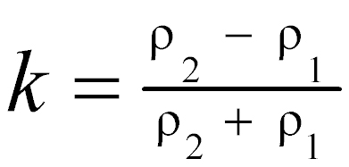
The simplest multilayer case is that of a single layer of finite thickness overlying a homogeneous half-space of different resistivity. The VES curves for this case vary in a relatively simple way, and a complete set of reference curves can be plotted on a single sheet of paper. Standard two-layer curves for the Schlumberger array are included in figure 7. The curves are plotted on a logarithmic scale, both horizontally and vertically, and are normalized by plotting the ratio of apparent resistivity to the first layer resistivity (ρa/ρ1) against the ratio of electrode spacing to the first layer thickness (a/d1). Each curve of the family represents one value of the parameter k, which is defined by
 (11)
(11)
The apparent resistivity for small electrode spacings approaches ρ1 and for large spacings approaches ρ2; these curves begin at ρa/ρ1 = 1, and asymptotically approach ρa/ρ1 = ρ2/ρ1.
Any two-layer curve for a particular value of k, or for a particular ratio of layer resistivities, must have the same shape on the logarithmic plot as the corresponding standard curve. It differs only by horizontal and vertical shifts, which are equal to the logarithms of the thickness and resistivity of the first layer. The early (i.e., corresponding to the smaller electrode spacings) portion of more complex multiple-layer curves can also be fitted to two-layer curves to obtain the first layer parameters ρ1 and d1 and the resistivity ρ2 of layer 2. The extreme curves in figure 7 correspond to values of k equal to 1.0 and -1.0; these values represent infinitely great resistivity contrasts between the upper and lower layers. The first case represents a layer 2 that is a perfect insulator; the second, a layer 2 that is a perfect conductor. The next nearest curves in both cases represent a ratio of 19 in the layer resistivities. Evidently, where the resistivity contrast is more than about 20 to 1, fine resolution of the layer 2 resistivity cannot be expected. Loss of resolution is not merely an effect of the way the curves are plotted, but is representative of the basic physics of the problem and leads to ambiguity in the interpretation of VES curves.
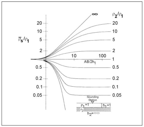
Figure 7. Two-layer master set of sounding curves for the Schlumberger array. (Zohdy 1974a, 1974b)
Where three or more strata of contrasting resistivity are present, the VES curves are more complex than the two-layer curves. For three layers, there are four possible types of VES curves, as shown in figure 8, depending on the nature of the successive resistivity contrasts. The classification of these curves is found in the literature with the notations H, K, A, and Q. These symbols correspond respectively to bowl-type curves, which occur with an intermediate layer of lower resistivity than layers 1 or 3; bell-type curves, where the intermediate layer is of higher resistivity; ascending curves, where resistivities successively increase; and descending curves, where resistivities successively decrease. With four layers, another curve segment is present, so that 16 curve types can be identified: HK for a bowl-bell curve, AA for a monotonically ascending curve, and so on.
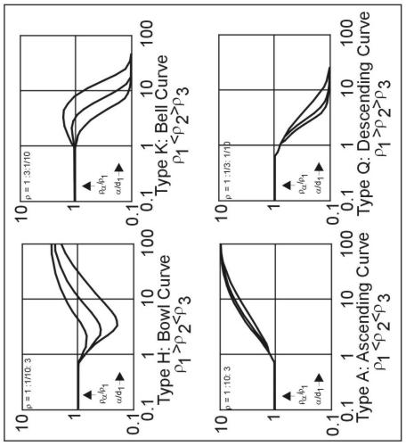
Figure 8. Four types of three-layer VES curves; the three sample curves for each of the four types represent values of d2/d1= 1/3, 1 and 3.
Before the availability of personal computers, the curve-matching process was done graphically by plotting the field data plotted on transparent log-log graph paper at the same scale of catalogs of two- and three-layer standard curves. The use of standard curves requires an identification of the curve type followed by a comparison with standard curves of that type to obtain the best match. Two-layer and three-layer curves can be used for complete interpretation of VES curves of more layers by the Auxiliary Point Method, which requires the use of a small set of auxiliary curves and some constructions. Discussions and step-by-step examples of this method are given by Zohdy (1965), Orellana and Mooney (1966), and Keller and Frischknecht (1966). Sets of standard curves have been developed by several workers. Orellana and Mooney (1966) published a set of 1,417 two-, three-, and four-layer Schlumberger curves, accompanied by a set of auxiliary curves, and tabulated values for both Schlumberger and Wenner curves. Apparent resistivity values for 102 three-layer Wenner curves were published by Wetzel and McMurray (1937). A collection of 2,400 two-, three-, and four-layer curves was published by Mooney and Wetzel (1956). Most, if not all, of these publications are out of print, but copies may be available in libraries.
Ghosh (1971a, 1971b) and Johansen (1975) used linear filter theory to develop a fast numerical method for computing apparent resistivity values from the resistivity transforms, and vice versa. With these methods, new standard curves or trial VES curves can be computed as needed, with a digital computer or a calculator, either to match the curves or to check the validity of an interpretation of the field data. Thus, trial-and-error interpretation of VES data is feasible. Trial values of the layer parameters can be guessed, checked with a computed apparent resistivity curve, and adjusted to make the field and computed curves agree. The process will be much faster, of course, if the initial guess is guided by a semiquantitative comparison with two- and three-layer curves. Computer programs have been written by Zohdy (1973, 1974a, 1975), Zohdy and Bisdorf (1975), and several commercial software companies for the use of this method to obtain the layer parameters automatically by iteration, starting with an initial estimate obtained by an approximate method. Most computer programs require a user-supplied initial estimate (model), whereas some programs can optionally generate the initial mode. After a suite of sounding curves have been individually interpreted in this manner, a second pass can be made where certain layer thicknesses and/or resistivities can be fixed to give a more consistent project-wide interpretation.
Interpretation of Horizontal Profiling Data
Data obtained from horizontal profiling for engineering applications are normally interpreted qualitatively. Apparent resistivity values are plotted and contoured on maps, or plotted as profiles, and areas displaying anomalously high or low values or anomalous patterns are identified. Interpretation of the data, as well as the planning of the survey, must be guided by the available knowledge of the local geology. The interpreter normally knows what he is looking for in terms of geological features and their expected influence on apparent resistivity, because the resistivity survey is motivated by geological evidence of a particular kind of exploration problem (e.g., karst terrain). The survey is then executed in a way that is expected to be most responsive to the kinds of geological or hydrogeological features sought. A pitfall inherent in this approach is that the interpreter may be misled by his preconceptions if he is not sufficiently alert to the possibility of the unexpected occurring. Alternative interpretations should be considered, and evidence from as many independent sources as possible should be applied to the interpretation. One way to help plan the survey is to construct model VES sounding curves for the expected models, vary each model parameter separately by say 20%, and then choose electrode separations that will best resolve the expected resistivity/depth variations. Most investigators then perform a number of VES soundings to verify and refine the model results before commencing horizontal profiling.
The construction of theoretical profiles is feasible for certain kinds of idealized models, and the study of such profiles is very helpful in understanding the significance of field profiles. Van Nostrand and Cook (1966) give a comprehensive discussion of the theory of electrical resistivity interpretation and numerous examples of resistivity profiles over idealized models of faults, dikes, filled sinks, and cavities.
Figure 9 illustrates a theoretical Wenner profile crossing a fault, a situation that can be thought of more generally as a survey line crossing any kind of abrupt transition between areas of different resistivity. The figure compares a theoretical curve, representing continuous variation of apparent resistivity with location of the center of the electrode array, and a theoretical field curve that would be obtained with an interval of a/2 between stations. More commonly, an interval equal to the electrode spacing would be used; various theoretical field curves for that case can be drawn by connecting points on the continuous curve at intervals of a. These curves would fail to reveal much of the detail of the continuous curve and could look quite different from one another. Figure 10 illustrates a profile across a shale-filled sink (i.e., a body of relatively low resistivity) and compares it `ith the theoretical continuous curve and a theoretical field curve. The theoretical curves are for a conductive body exposed at the surface, while the field case has a thin cover of alluvium, but the curves are very similar. Figure 9a shows a number of theoretical continuous profiles across buried perfectly insulating cylinders. This model would closely approximate a subsurface tunnel and less closely an elongated cavern. A spherical cavern would produce a similar response but with less pronounced maxima and minima. Figure 11b shows a set of similar curves for cylinders of various resistivity contrasts.
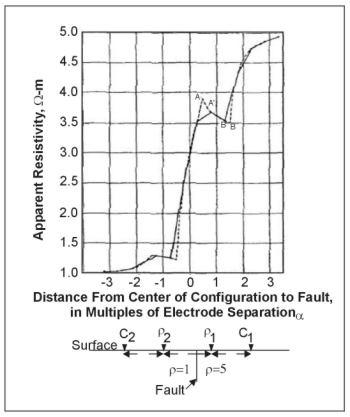
Figure 9. Wenner horizontal resistivity profile over a vertical fault; typical field curve (solid line), theoretical curve (dashed line). (Van Nostrand and Cook 1966)
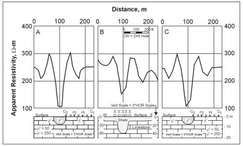
Figure 10. Wenner horizontal resistivity profiles over a filled sink: A) continuous theoretical curve over hemispherical sink, b) observed field curve with geologic cross section, c) theoretical field plot over hemispherical sink (Van Nostrand and Cook 1966).
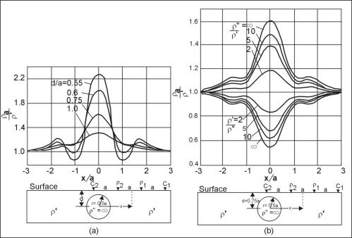
Figure 11. Theoretical Wenner profiles across a circular cylinder; a) perfectly insulating cylinders at different depths, b) cylinders of different resistivity contrasts. (Van Nostrand and Cook 1966)
2D & 3D Electrical Imaging
Following on the 1D applications of resistivity imaging theory, comes the 2D and subsequently 3D applications. The 2D profiles take the above sounding techniques and integrate them into a 2D plane transecting the desired target area. The most common configuration of the 2D survey employs dipole-dipole electrode configurations. An example of the data aquisition geometry for a 2D profile is presented in figure 12.
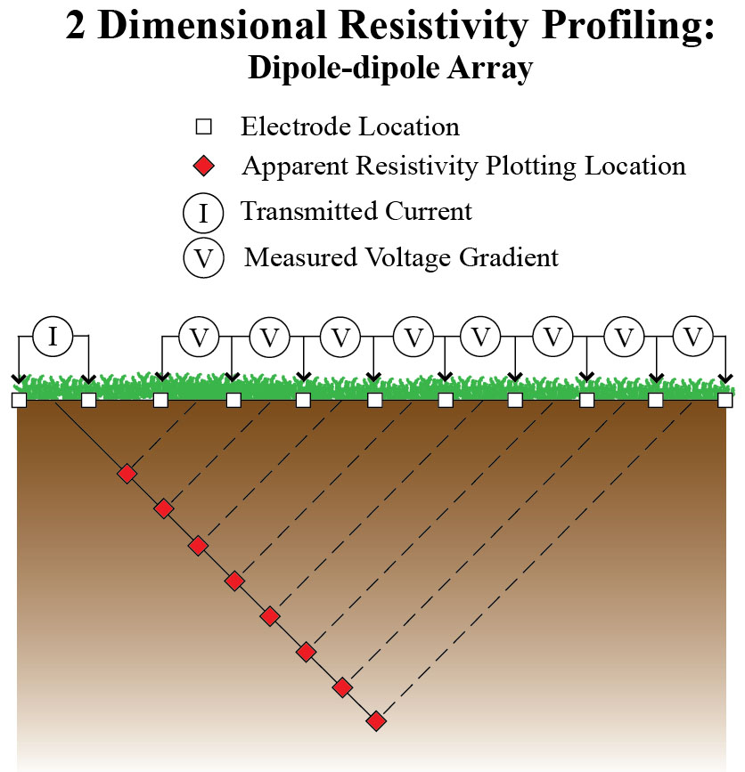
Figure 12. Two dimensional measurement configuration for a dipole-dipole resistivity profile. Pseudosection plotting location indicated inred.
Figure 12 shows a transmitting current dipole (I) followed by a series of potential dipoles (V) which measure the resulting voltage gradient at each station along the line. Subsequent measurements are completed by sequentially moving the current dipole down the line. However, alternative resistivity measurements can be made using towed surface or marine arrays, which would maintain the above configuration, and build up the 2D image by moving the entire measurement array for each series of measurements. In both cases the resulting image plots the apparent resistivity with depth, which is then contoured (commonly krigged) using a commercially available program. The color contoured image displays the distribution of apparent resistivity values and associated gradients within the area of interest. In order to convert the apparent resistivity data to true resistivity, the data are inverted. Figure 13 displays an example of a measured apparent resistivity pseudosection at the top, followed by a calculated apparent resistivity pseudosection, and resulting in the inverted true resistivity 2D section. The numbers presented at the bottom of the inverted section display goodness of fit criteria used to assess the accuracy of the calculated resistivity model. Finally note that the surface elevations have been included in the final model, accounting for variations in measurement geometry due to changing topography.
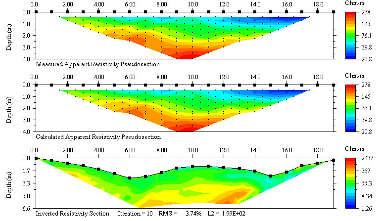
Figure 13. Examples of measured apparent resistivity, calculated apparent resistivity, and inverted resistivity sections (http://www.agiusa.com/agi2dimg.shtml). This image is provided for demonstration purposes, and is not intended as an endorsement for use of this software.
Figure 14 presents an alternative way of generating a 2D electrical resistivity image of the subsurface. In this scenario a series of elelctrodes are placed at equavalent intervals vertically down two well casings. Each available dipole is used for both transmitting (current) and receiving (voltage). Figure 15 shows an example of an inverted 2D cross borehole ERT data set.
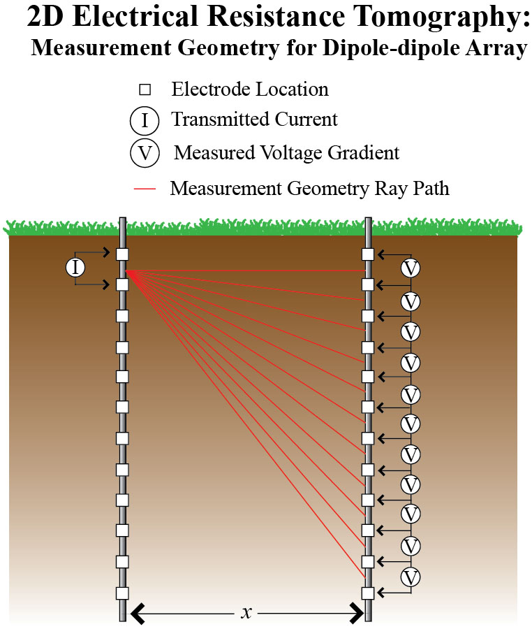
Figure 14. The measurement ray paths associated with a single cross borehole transmitting dipole. Traditionally the measuremnts are acquired using each available dipole as both a transmitting and receiving dipole.
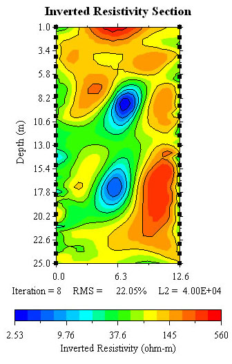
Figure 15. An example of an inverted cross borehole ERT data set (http://www.agiusa.com/agi2dimg.shtml).This image is provided for demonstration purposes, and is not intended as an endorsement for use of this software.
The pages found under Surface Methods and Borehole Methods are substantially based on a report produced by the United States Department of Transportation:
Wightman, W. E., Jalinoos, F., Sirles, P., and Hanna, K. (2003). "Application of Geophysical Methods to Highway Related Problems." Federal Highway Administration, Central Federal Lands Highway Division, Lakewood, CO, Publication No. FHWA-IF-04-021, September 2003. http://www.cflhd.gov/resources/agm/![]()