Magnetic Methods
Basic Concepts
The Earth possesses a magnetic field caused primarily by sources in the core. The form of the field is roughly the same as would be caused by a dipole or bar magnet located near the Earth's center and aligned sub parallel to the geographic axis. The intensity of the Earth's field is customarily expressed in S.I. units as nanoteslas (nT) or in an older unit, gamma (γ): 1 γ = 1 nT = 10-3 μT. Except for local perturbations, the intensity of the Earth's field varies between about 25 and 80 μT over the conterminous United States.
Many rocks and minerals are weakly magnetic or are magnetized by induction in the Earth's field, and cause spatial perturbations or "anomalies" in the Earth's main field. Man-made objects containing iron or steel are often highly magnetized and locally can cause large anomalies up to several thousands of nT. Magnetic methods are generally used to map the location and size of ferrous objects. Determination of the applicability of the magnetics method should be done by an experienced engineering geophysicist. Modeling and incorporation of auxiliary information may be necessary to produce an adequate work plan.
Theory
The Earth's magnetic field dominates most magnetic measurements made at or near the surface of the Earth. The Earth's total field intensity varies considerably by location over the surface of the Earth. Most materials except for permanent magnets, exhibit an induced magnetic field due to the behavior of the material when the material is in a strong field such as the Earth's. Induced magnetization (sometimes called magnetic polarization) refers to the action of the field on the material wherein the ambient field is enhanced causing the material itself to act as a magnet. The field caused by such a material is directly proportional to the intensity of the ambient field and to the ability of the material to enhance the local field--a property called magnetic susceptibility. The induced magnetization is equal to the product of the volume magnetic susceptibility and the inducing field of the Earth:
![]() (1)
(1)
where
For most materials, k is much less than 1 and, in fact, is usually of the order of 10-6 for most rock materials. The most important exception is magnetite whose susceptibility is about 0.3. From a geologic standpoint, magnetite and its distribution determine the magnetic properties of most rocks. There are other important magnetic minerals in mining prospecting, but the amount and form of magnetite within a rock determines how most rocks respond to an inducing field. Iron, steel, and other ferromagnetic alloys have susceptibilities one to several orders of magnitude larger than magnetite. The exception is stainless steel, which has a small susceptibility.
The importance of magnetite cannot be exaggerated. Some tests on rock materials have shown that a rock containing 1% magnetite may have a susceptibility as large as 10-3, or 1,000 times larger than most rock materials. Table 1 provides some typical values for rock materials. Note that the range of values given for each sample generally depends on the amount of magnetite in the rock.
Table 1. Approximate magnetic susceptibility of representative rock types.
|
Rock Type |
Susceptibility (k) |
|
Altered ultra basics |
10-4 to 10-2 |
|
Basalt |
10-4 |
|
Gabbro |
10-4 to 10-3 |
|
Granite |
10-5 to 10-3 |
|
Andesite |
10-4 |
|
Rhyolite |
10-5 to 10-4 |
|
Metamorphic rocks |
10-4 to 10-6 |
|
Most sedimentary rocks |
10-6 to 10-5 |
|
Limestone and chert |
10-6 |
|
Shale |
10-5 to 10-4 |
Thus, it can be seen that in most engineering and environmental scale investigations, the sedimentary and alluvial sections will not show sufficient contrast such that magnetic measurements will be of use in mapping the geology. However, the presence of ferrous materials in ordinary municipal trash and in most industrial waste does allow the magnetometer to be effective in direct detection of landfills. Other ferrous objects, which may be detected, include pipelines, underground storage tanks, and some ordnance.
Instrumentation
There are many different types of magnetometers in use today for varrying purposes. For enviromental and engineering investigations the current standards are generally proton procession and cesium vapor. The magnetometer type reflects the physical process by which the magnetic field is measured. Proton procession instruments have a sensor filled with a hydrogen rich fluid (similar to kerosene). An inductor creates a strong magnetic field in the fluid resulting in the allignment of protons. When the inducted current is suspended, the relaxation rate as the protons return to ambient magnetic conditions is recorded. This rate is directly proportional to the magnetic field. An overhauser magnetometer, presents a variaition on the proton procession magnetometer by using radio frequency magnetic fields to generate the polarizing signal. This improves the results of a proton procession magnetometer, as the RF field does not interfer with the precession signal.
A cesium vapor magentometer is usually made up of a photon emitter, an absorption chamber, a buffer gas, and a photon detector. The known properties of a cesium atom allow for the displacement of electrons by applying photons. Cesium can exist at any of nine energy levels; however, it is only affected by the photons at three of the nine energy levels. Therefore, eventually photons will pass thorugh the cesium vapor unhindered, no longer resulting in transfer of electrons. This is essentially the "zeroed" state or baseline, by which relative subsequent measurements are made. Then, when an external AC magnetic field is applied, the difference in energy levels of the electrons is established by the ambient magnetic field. The new field allows photons to transfer electrons once again, which is measured by the amount of light reaching the photon detector. Resulting in a high performance magnetometer.
Given the requirements for high data density and high aquisition rate, the cesium vapor approach is generally more favorable due to the faster measurement speed. Proton procession magnetometers are frequently incorporated as base stations in these types of investigations. Figure 1 displays a common base station configuration (proton procession) as well as a common rover configuration (gradiometry).
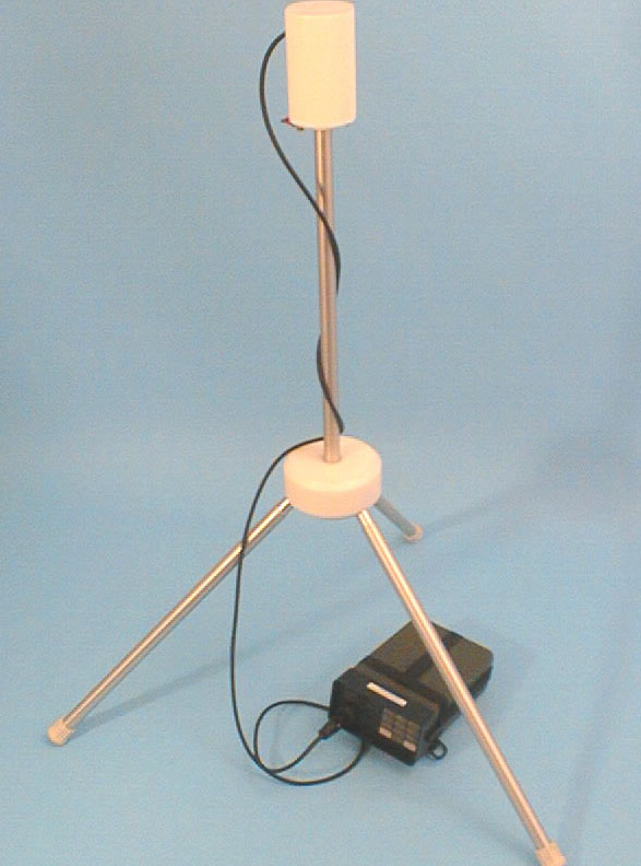
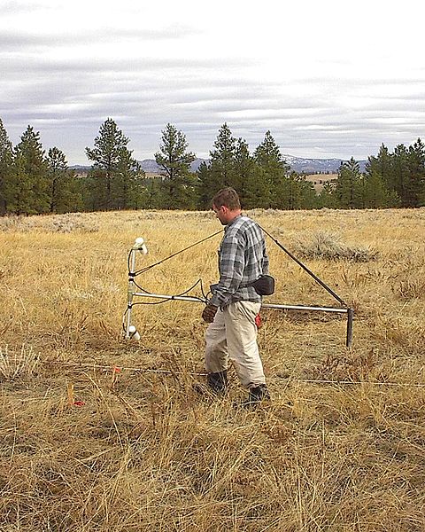
Figure 1. Geometrics G856 Proton procession magnetomter in base station mode (image from: ftp://geom.geometrics.com/pub/mag/Manuals/856Manual.pdf), and G858 cesium vapor magnetometer, in gradiometry configuration (image from: http://commons.wikimedia.org/wiki/File:Mag_survey_g858grad.JPG). Images are presented for demonstration purposes only, the EPA does not endorse use of the above products.
Data Acquisition
Ground magnetic measurements are usually made with portable instruments at regular intervals along more or less straight and parallel lines that cover the survey area. Often the interval between measurement locations (stations) along the lines is less than the spacing between lines.
The magnetometer is a sensitive instrument that is used to map spatial variations in the Earth's magnetic field. In the proton magnetometer, a magnetic field that is not parallel to the Earth's field is applied to a fluid rich in protons causing them to partly align with this artificial field. When the controlled field is removed, the protons tend to return to its original direction in the earth's magnetic field by precessing around the Earth's field at a frequency depending on the intensity of the Earth's field. By measuring this precession frequency, the total intensity of the field can be determined. The physical basis for several other magnetometers, such as the cesium or rubidium-vapor magnetometers, is similarly founded in a fundamental physical constant. The optically pumped magnetometers have increased sensitivity and shorter cycle times (as small as 0.04 s), making them particularly useful in airborne applications.
The incorporation of computers and non-volatile memory in magnetometers has greatly increased their ease of use and data handling capability. The instruments typically will keep track of position, prompt for inputs, and internally store the data for an entire day of work. Downloading the information to a personal computer is straightforward, and plots of the day's work can be prepared each night.
To make accurate anomaly maps, temporal changes in the Earth's field during the period of the survey must be considered. Normal changes during a day, sometimes called diurnal drift, are a few tens of nT, but changes of hundreds or thousands of nT may occur over a few hours during magnetic storms. During severe magnetic storms, which occur infrequently, magnetic surveys should not be made. The correction for diurnal drift can be made by repeat measurements of a base station at frequent intervals. The measurements at field stations are then corrected for temporal variations by assuming a linear change of the field between repeat base station readings. Continuously recording magnetometers can also be used at fixed base sites to monitor the temporal changes. If time is accurately recorded at both base site and field location, the field data can be corrected by subtraction of the variations at the base site.
The base-station memory magnetometer, when used, is set up every day prior to collection of the magnetic data. Ideally the base station is placed at least 100 m from any large metal objects or traveled roads and at least 500 m from any power lines when feasible. The base station location must be very well described in the field book, as others may have to later locate it based on the written description.
Some QC/QA procedures require that several field-type stations be occupied at the start and end of each day's work. This procedure indicates that the instrument is operating consistently. Where it is important to be able to reproduce the actual measurements on a site exactly (such as in certain forensic matters), an additional procedure is required. The value of the magnetic field at the base station must be asserted (usually a value close to its reading on the first day) and each day's data corrected for the difference between the asserted value and the base value read at the beginning of the day. As the base may vary by 10 to 25 nT or more from day to day, this correction ensures that another person using the same base station and the same asserted value will get the same readings at a field point to within the accuracy of the instrument. This procedure is always good technique but is often neglected by persons interested in only very large anomalies (> 500 nT, etc.).
Intense fields from man-made electromagnetic sources can be a problem in magnetic surveys. Most magnetometers are designed to operate in fairly intense 60-Hz and radio frequency fields. However, extremely low frequency fields caused by equipment using direct current or the switching of large alternating currents can be a problem. Pipelines carrying direct current for cathodic protection can be particularly troublesome. Although some modern ground magnetometers have a sensitivity of 0.1 nT, sources of cultural and geologic noise usually prevent full use of this sensitivity in ground measurements.
After all corrections have been made, magnetic survey data are usually displayed as individual profiles or as contour maps. Identification of anomalies caused by cultural features, such as railroads, pipelines, and bridges is commonly made using field observations and maps showing such features. For some purposes, a close approximation of the gradient of the field is determined by measuring the difference in the total field between two closely spaced sensors. The quantity measured most commonly is the vertical gradient of the total field.
The magnetometer is operated by a single person. However, grid layout, surveying, or the buddy system may require the use of another technician. If two magnetometers are available, production is usually doubled as the ordinary operation of the instrument itself is straightforward.
One way of limiting noise, compensating for temporal variablility in the earths magnetic field, and enhancing small anomalies is to complete a gradiometry survey. A gradiometer is simply a magentometer with two or more sensors spaced at a constant known separation. By measuring essentially the same values at two different distances from the intended targets (the gradient of the earths magnetic field at those points), and subtracting the measurements, smaller signals are enhanced.
Distortion
Steel and other ferrous metals in the vicinity of a magnetometer can distort the data. Large belt buckles, etc., must be removed when operating the unit. A compass should be more than 3 m away from the magnetometer when measuring the field. A final test is to immobilize the magnetometer and take readings while the operator moves around the sensor. If the readings do not change by more than 1 or 2 nT, the operator is "magnetically clean." Zippers, watches, eyeglass frames, boot grommets, room keys, and mechanical pencils can all contain steel or iron. On very precise surveys, the operator effect must be held under 1 nT.
To obtain a representative reading, the sensor should be operated well above the ground. This procedure is done because of the probability of collections of soil magnetite disturbing the reading near the ground. In rocky terrain where the rocks have some percentage of magnetite, sensor heights of up to 4 m have been used to remove near-surface effects. One obvious exception to this is some types of ordnance detection where the objective is to detect near-surface objects. Often a rapid-reading magnetometer is used (cycle time less than 1/4 s) and the magnetometer is used to sweep across an area near the ground. Small ferrous objects can be detected, and spurious collections of soil magnetite can be recognized by their lower amplitude and dispersion. Ordnance detection requires not only training in the recognition of dangerous objects, but also experience in separating small, intense, and interesting anomalies from more dispersed geologic noise.
Data recording methods will vary with the purpose of the survey and the amount of noise present. Methods include taking three readings and averaging the results, taking three readings within a meter of the station and either recording each or recording the average. Some magnetometers can apply either of these methods and even do the averaging internally. An experienced field geophysicist will specify which technique is required for a given survey. In either case, the time of the reading is also recorded unless the magnetometer stores the readings and times internally.
Sheet‑metal barns, power lines, and other potentially magnetic objects will occasionally be encountered during a magnetic survey. When taking a magnetic reading in the vicinity of such items, describe the interfering object and note the distance from it to the magnetic station in your field book.
Items to be recorded in the field book for magnetics include:
a) Station location, including locations of lines with respect to permanent landmarks or surveyed points.
b) Magnetic field and/or gradient reading.
c) Time.
d) Nearby sources of potential interference.
The experienced magnetics operator will be alert for the possible occurrence of the following:
1. Excessive gradients may be beyond the magnetometer's ability to make a stable measurement. Modern magnetometers give a quality factor for the reading. Multiple measurements at a station, minor adjustments of the station location and other adjustments of technique may be necessary to produce repeatable, representative data.
2. Nearby metal objects may cause interference. Some items, such as automobiles, are obvious, but some subtle interference will be recognized only by the imaginative and observant magnetics operator. Old buried curbs and foundations, buried cans and bottles, power lines, fences, and other hidden factors can greatly affect magnetic readings.
Data Processing and Interpretation
Total magnetic disturbances or anomalies are highly variable in shape and amplitude; they are almost always asymmetrical, sometimes appear complex even from simple sources, and usually portray the combined effects of several sources. An infinite number of possible sources can produce a given anomaly, giving rise to the term ambiguity.
One confusing issue is the fact that most magnetometers used measure the total field of the Earth: no oriented system is recorded for the total field amplitude. The consequence of this fact is that only the component of an anomalous field in the direction of Earth's main field is measured. Figure 1 illustrates this consequence of the measurement system. Anomalous fields that are approximately perpendicular to the Earth's field are undetectable.
Additionally, the induced nature of the measured field makes even large bodies act as dipoles, that is, like a large bar magnet. If the (usual) dipolar nature of the anomalous field is combined with the measurement system that measures only the component in the direction of the Earth's field, the confusing nature of most magnetic interpretations can be appreciated.
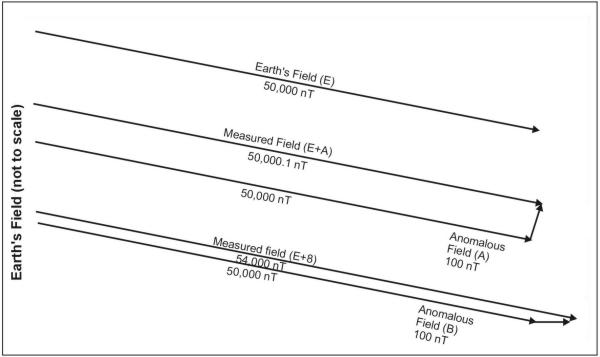
Figure 2. Magnetic field vector examples for two anomalous fields.
Data Processing and Interpretation
To achieve a qualitative understanding of what is occurring, consider figure 2. Within the contiguous United States, the magnetic inclination, that is the angle the main field makes with the surface, varies from 55 to 70 degrees. The figure illustrates the field associated with the main field, the anomalous field induced in a narrow body oriented parallel to that field, and the combined field that will be measured by the total-field magnetometer. The scalar values that would be measured on the surface above the body are listed. From this figure, one can see how the total-field magnetometer records only the components of the anomalous field.
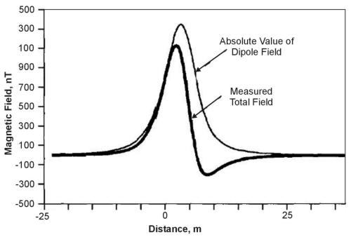
Figure 2. Actual and measured fields due to magnetic
inclination.
Two Dimensional Imaging
The techniques presented above can be applied to two dimensional imaging by conducting a series of parallel transects, correcting for heading error, and contouring the data. Figure 3 presents the results of a case study where total field and gradiometry magentic data were acquired in an effort to characterize the subsurface metal infrastructure at a former radio active waste disposal site. The hatched lines represent the known outline of the burial cribs and trenches, while the alternating red and blue dipolar features are indicative of the metallic pipelines and associated infrastructure used to transport liquid waste to the disposal facilities. Lastly, the separate large red nonlinear anomalies indicate steel monitoring well locations.
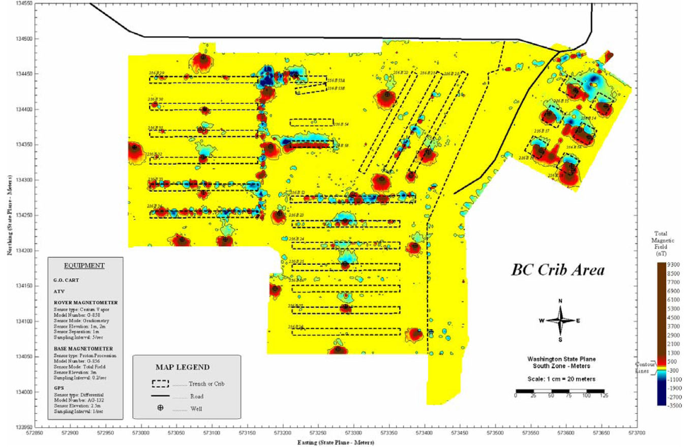
Figure 3. Total magnetic field data for the BC Cribs and Trenches site at the Department of Energy Hanford Nuclear Waste Reservation, WA ( Rucker & Sweeney, 2004).
The pages found under Surface Methods and Borehole Methods are substantially based on a report produced by the United States Department of Transportation:
Wightman, W. E., Jalinoos, F., Sirles, P., and Hanna, K. (2003). "Application of Geophysical Methods to Highway Related Problems." Federal Highway Administration, Central Federal Lands Highway Division, Lakewood, CO, Publication No. FHWA-IF-04-021, September 2003. http://www.cflhd.gov/resources/agm/![]()