[Note to the reader: This document has been slightly reformatted
for ease of use on the Internet. Since this document was retyped
from the published version, it is possible there are errors. If
you find any errors, please report them to Barry Gilbert (gilbert.barry@epamail.epa.gov)
]
OAQPS GUIDELINES SERIES
The guideline series of reports is being issued by the Office of
Air Quality Planning and Standards (OAQPS) to provide information
to state and local air pollution control agencies, for example,
to provide guidance on the acquisition and processing of air quality
data and on the planning and analysis requisite for the maintenance
of air quality. Reports published in this series will be available
as supplies permit - from the Library Services Office (MD-35), U.S.
Environmental Protection Agency, Research Triangle Park, North Carolina
27711; or for a nominal fee, from the National Technical Information
Service, 5285 Port Royal Road, Springfield, Virginia 22161.
Publication No. EPA-450/4-79-003
OAQPS No. 1.2-108

Table of Contents

1.	INTRODUCTION
		1.1	Background
		1.2	Terminology
  		1.3	Basic Premises

2.	ASSESSING COMPLIANCE
		2.1	Interpretation of "Expected Number"
		2.2	Estimating Exceedances for the Year
		2.3	Extension to Multiple Years
		2.4	Example Calculation

3.	ESTIMATING DESIGN VALUES
		3.1	Discussion of Design Values
		3.2	The Use of Statistical Distributions
		3.3	Methodologies
		3.4	Quick Test for Design Values
		3.5	Discussion of Data Requirements
		3.6	Example Design Value Computations

4.	APPLICATIONS WITH LIMITED AMBIENT DATA

5.	REFERENCES
1. INTRODUCTION
The ozone National Ambient Air Quality Standards (NAAQS) contain
the phrase "expected number of days per calendar year." [1] This
differs from the previous NAAQS for photochemical oxidants which
simply state a particular concentration "not to be exceeded more
than once per year." [2] The data analysis procedures to be used
in computing the expected number are specified in Appendix H to
the ozone standard. The purpose of this document is to amplify the
discussions contained in Appendix H dealing with compliance assessment
and to indicate the data analysis procedures necessary to determine
appropriate design values for use in developing control strategies.
Where possible, the approaches discussed here are conceptually similar
to the procedures presented in the earlier "Guideline for Interpreting
Air Quality Data With Respect to the Standards" (ALPS 1.2-008, revised
February, 1977). [3] However, the form of the ozone standards necessitates
certain modifications in two general areas: (1) accounting for less
than complete sampling and (2) incorporating data from more than
one year.
Although the interpretation of the proposed standards may initially
appear complicated, the basic principle is relatively straightforward.
In general, the average number of days per year above the level
of the standard must be less than or equal to 1. In its simplest
form, the number of exceedances each year would be recorded and
then averaged over the past three years to determine if this average
is less than or equal to 1. Most of the complications that arise
are consequences of accounting for incomplete sampling or changes
in emissions.
Throughout the following discussion certain points are assumed
that are consistent with previous guidance [3] but should be reiterated
here for completeness. The terms hour and day (daily) are interpreted
respectively as clock hour and calendar day. Air quality data are
examined on a site by site basis and each individual site must meet
the standard. In general, data from several different sites are
not combined or averaged when performing these analyses. These points
are discussed in more detail elsewhere. [3]
This document is organized so that the remainder of this introductory
section presents the background of the problem, terminology, and
certain basic premises that were used in developing this guidance.
This is followed by a section which examines methods for determining
appropriate design values. The final section discusses approaches
that might be employed in cases without ambient monitoring data.
This last section is brief and fairly general, because it treats
an aspect of the problem which would be expected to rapidly evolve
once these two forms of the NAAQS become established. In several
parts of this document the material is developed in a conversational
format in order to highlight certain points.
1.1. Background
The previous National Ambient Air Quality Standard (NAAQS) for
oxidant stated that no more than one hourly value per year should
exceed 160 micrograms per cubic meter (.08 ppm). [2] With this type
of standard, the second highest value for the year becomes the decision-making
value. If it is above 160 micrograms per cubic meter then the standard
was exceeded. This would initially appear to be an ideal type of
standard. The wording is simple and the interpretation is obvious-or
is it? Suppose the second highest value for the year is less than
160 micrograms per cubic meter and the question asked is, "Does
this site meet the standard?" An experienced air pollution analyst
would almost automatically first ask, "How many observations were
there?" This response reflects the obvious fact that the second
highest measured value can depend upon how many measurements were
made in the year. Carried to the absurd, if only one measurement
is made for the year, it is impossible to exceed this type of standard.
Obviously, this extreme case could be remedied by requiring some
minimum number of measurements per year. However, the basic point
is that the probability of detecting a violation would still be
expected to increase as the number of samples increased from the
specified minimum to the maximum possible number of observations
per year. Therefore, the present wording of this type of standard
inherently penalizes an area that performs more than the minimum
acceptable amount of monitoring. Furthermore, the specification
of a minimum data completeness criterion still does not solve the
problem of what to do with those data sets that fail to meet this
criterion.
A second problem with the current wording of the standard is not
as obvious but becomes more apparent when considering what is involved
in maintaining the standard year after year. For example, suppose
an area meets the standard in the sense that only one value for
the year is above 160 micrograms per cubic meter. Because of the
variability associated with air quality data, the fact that one
value is above the standard level means that there is a chance that
two values could be above this standard level the next year even
though there is no change in emissions. In other words, any area
with emissions and meteorology that can produce one oxidant value
above the standard has a definite risk of sometime having at least
two such values occurring in the same year and thereby violating
the standard. This situation may be viewed as analogous to the "10
year flood" and "100 year flood" concepts used in hydrology; i.e.,
high values may occur in the future but the likelihood of such events
is relatively low. However, with respect to air pollution, any rare
violation poses distinct practical problems. From a control agency
viewpoint, the question arises as to what should be done about such
a violation if it is highly unlikely to reoccur in the next few
years. If the decision is made to ignore such a violation then the
obvious implication is that the standard can occasionally be ignored.
This is not only undesirable but produces a state of ambiguity that
must be resolved to intelligently assess the risk of violating the
standard. In other words, some quantification is needed to describe
what it means to maintain the standard year after year in view of
the variation associated with air quality data. The wording of the
ozone standard is intended to alleviate these problems.
1.2. Terminology
The term "daily maximum value" refers to the maximum hourly ozone
value for a day. As defined in Appendix H, a valid daily maximum
means that at least 75% of the hourly values from 9:01 A.M. to 9:00
P.M. (LST) were measured or at least one hourly value exceeded the
level of the standard. This criterion is intended to reflect adequate
monitoring of the daylight hours while allowing time for routine
instrument maintenance. The criterion also ensures that high hourly
values are not omitted merely because too few values were measured.
It should be noted that this is intended as a minimal criterion
for completeness and not as a recommended monitoring schedule.
A final point worth noting concerns terminology. The term "exceedance"
is used throughout this document to describe a daily maximum ozone
measurement that is above the level of the standard. Therefore the
phrase "expected number of exceedances" is equivalent to "the expected
number of daily maximum ozone values above the level of the standard."
1.3. Basic Premises
By its very nature, the existence of a guideline document implies
several things: (1) that there is a problem, (2) that a solution
is provided, and (3) that there were several alternatives considered
in reaching the solution. Obviously, if there is no problem then
the guideline is of limited value, and if there were not some alternative
solutions then the guidance is perhaps superfluous or at best educational.
The third point indicates that the "best" alternative, in some sense,
was selected. With this in mind, it is useful to briefly discuss
some of the key points that were considered in judging the various
options. The purpose of this section is to briefly indicate the
criteria used in developing this particular guideline.
The most obvious criterion is simplicity. This simplicity extends
to several aspects of the problem. When someone asks if a particular
area meets the standard they expect either a "yes" or "no" as the
answer or even an occasional "I don't know". Secondly, this simplicity
should extend to the reason why the standard was met or violated.
If a panel of experts is required to debate the probability that
an area is in compliance then the general public may rightly feel
confused about just what is being done to protect their health.
Also, the more clear-cut the status of an area is (and the reasons
why) the more likely it is that all groups involved can concentrate
on the real problem of maintaining clean air rather than arguing
over minor side issues.
While simplicity is desirable, if the problem is complex the solution
cannot be oversimplified. In other words, the goal is to develop
a solution that is simple and yet not simple-minded. In order to
do this, the approach taken in this document is to recognize that
there are two questions involved in determining compliance: (1)
was the standard violated? and (2) if so, by how much? The first
question is the simpler of the two in that a "yes/no" answer is
expected. The second question implies both a quantification and
a determination of what to do about it. Therefore, it seems reasonable
to have a more complicated procedure for determining the second
answer.
In addition to the trade-offs between simplicity and complexity
another problem is to allow a certain amount of flexibility without
being vague. There are several reasons for allowing some degree
of flexibility. Not only do available resources vary from one area
to another but the complexity of the air pollution problems vary.
An area with no pollution problem should not be required to do an
extensive analysis just because that level of detail is needed someplace
else. Conversely, an area with sufficient resources to perform a
detailed analysis of their pollution problem to develop an optimum
control strategy should not be constrained from doing so simply
because it is not warranted elsewhere. Furthermore, a certain degree
of flexibility is essential to allow for modified monitoring schedules
that are used to make the best use of available resources.
In addition to these points concerning simplicity and flexibility,
certain other considerations are of course involved. In particular,
the methodology employed cannot merely ignore high values for a
particular year simply because they are unlikely to reoccur. The
purpose of the standard is to protect against high values in a manner
consistent with the likelihood of their occurrence.
A final point is that the proposed interpretation should involve
a framework that could eventually be extended to other pollutants,
if necessary, and easily modified in the future as our knowledge
and understanding of air pollution increases.
It should be noted that no specific mention is made of measurement
error in the following discussions. While it would be naive to assume
that measurement errors do not occur, at the present time it is
difficult to allow for measurement errors in a manner that is not
tantamount to re-defining the level of the standard. Obviously,
there is no question that data values known to be grossly in error
should be corrected or eliminated. In fact, the use of multiple
years of data for the ozone standards should facilitate this process.
The more serious practical problem is with the level of uncertainty
associated with every individual measurement. The viewpoint taken
here is that these inherent accuracy limitations are accounted for
in the choice of the level of the standard and that equitable risk
from one area to another is assured by use of the reference (or
an equivalent) ambient monitoring method and adherence to a required
minimum quality assurance program. It should be noted that the stated
level of the standard is taken as defining the number of significant
figures to be used in comparisons with the standard. For example,
a standard level of .12 ppm means that measurements are to be rounded
to two decimal places (.005 rounds up), and, therefore, .125 ppm
is the smallest concentration value in excess of the level of the
standard.
2. ASSESSING COMPLIANCE
This section examines the ozone standard with particular attention
given to the evaluation of compliance. This is done in several steps.
The first is a discussion of the term "expected number." Once this
is defined it is possible to consider the interpretation when applied
to several years of data or to less than complete sampling data.
An example calculation is included at the end of this section to
summarize and illustrate the major points.
2.1 Interpretation of "Expected Number"
The wording of the ozone standard states that the "expected number
of days per calendar year", must be "equal to or less than 1." The
statistical term "expected number" is basically an arithmetic average.
Perhaps the simplest way to explain the intent of this wording is
to give an example of what it would mean for an area to be in compliance
with this type of standard. Suppose an area has relatively constant
emissions year after year and its monitoring station records an
ozone value for every day of the year. At the end of each year,
the number of daily values above the level of the standard is determined
and this is averaged with the results of previous years. As long
as this arithmetic average remains "less than or equal to 1" the
area is in compliance. As far as rounding conventions are concerned,
it suffices to carry one decimal place when computing the average.
For example, the average of the three numbers, 1, 1, 2 is 1.3 which
is greater than 1.
Two features in this example warrant additional discussion to
clearly define how this proposal would be implemented. The example
assumes that a daily ozone measurement is available for each day
of the year so that the number of exceedances for the year is known.
On a practical basis this is highly unlikely and, therefore, it
will be necessary to estimate this quantity. This is discussed in
section 2.2. In the example, it is also assumed that several years
of data are available and there is relatively little change in emissions.
This is discussed in more detail in section 2.3.
The key point in the example is that as data from additional years
are incorporated into the average this expected number of exceedances
per year should stabilize. If unusual meteorology contributes to
a high number of exceedances for a particular year, then this will
be averaged out by the values for other "normal" years. It should
be noted that these high values would, therefore, not be ignored
but rather their relative contribution to the overall average is
in proportion to the likelihood of their occurrence. This use of
the average may be contrasted with an approach based upon the median.
If the median were used then the year with the greatest number of
exceedances could be ignored and there would be no guarantee of
protection against their periodic reoccurrence.
2.2 Estimating Exceedances for a Year
As discussed above, it is highly unlikely that an ozone measurement
will be available for each day of the year. Therefore, it will be
necessary to estimate the number of exceedances in a year. The formula
to be used for this estimation is contained in Appendix H of the
ozone standard. The purpose of this section is to present the same
basic formula but to expand upon the rationale for choosing this
approach and to provide illustrations of certain points.
Throughout this discussion the term "missing value" is used in
the general sense to describe all days that do not have an associated
ozone measurement. It is recognized that in certain cases a so-called
"missing value" occurs because the sampling schedule did not require
a measurement for that particular day. Such missing values, which
can be viewed as "scheduled missing values," may be the result of
planned instrument maintenance or, for ozone, may be a consequence
of a seasonal monitoring program. In order to estimate the number
of exceedances in a particular year it is necessary to account for
the possible effect of missing values. Obviously, allowance for
missing values can only result in an estimated number of exceedances
at least as large as the observed number. From a practical viewpoint,
this means that any site that is in violation of the standard based
upon the observed number of exceedances will not change status after
this adjustment. Thus, in a sense, this adjustment for missing values
is required to demonstrate attainment, but may not be necessary
to establish non-attainment.
In estimating the number of exceedances in cases with missing
data, certain practical considerations are appropriate. In some
areas, cold weather during the winter makes it very unlikely that
high ozone values would occur. Therefore, it is possible to discontinue
ozone monitoring in some localities for limited time periods with
little risk of incorrectly assessing the status of the area. As
indicated in Appendix H, the proposed monitoring regulations (CFR58)
would permit the appropriate Regional Administrator to waive any
ozone monitoring requirements during certain times of the year.
Although data for such a time period would be technically missing,
the estimation formula is structured in terms of the required number
of monitoring days and therefore these missing days would not affect
the computations.
Another point is that even though a daily ozone value is missing,
other data might indicate whether or not the missing value would
have been likely to exceed the standard level. There are numerous
ways additional information such as solar radiation, temperature,
or other pollutants could be used but the final result should be
relatively easy to implement and not create an additional burden.
An analysis of 258 site-years of ozone/oxidant data from the highest
sites in the 90 largest Air Quality Control Regions showed that
only 1% of the time did the high value for a day exceed .12 ppm
if the adjacent daily values were less than .09 ppm. With this in
mind the following exclusion of criterion may be used for ozone:
A missing daily ozone value may be assumed to be less than the
level of the standard if the daily maxima on both the preceding
day and the following day do not exceed 75% of the level of the
standard.
It should be noted that to invoke this exclusion criterion data
must be available from both adjacent days. Thus it does not apply
to consecutive missing daily values. Having defined the set of missing
values that may be assumed to be less than the standard it is possible
to present the computations required to adjust for missing data.
Let z denote the number of missing values that may be assumed
to be less than the standard. Then the following formula shall be
used to estimate the number of exceedances for the year:
	e=v+(v/n)*(N-n-z)		(1)
	          (* indicates multiplication)

	Where N =  the number of required monitoring days in the year

 	n  = the number of valid daily maxima

	v  = the number of measured daily values above the level of the standard

	z  = the number of days assumed to be less than the standard level, and

	e  = the estimated number of exceedances for the year.
This estimated number of exceedances shall be rounded to one decimal
place (fractional parts equal to .05 round up).
Note that N is always equal to the number of days in the year
unless a monitoring waiver has been granted by the appropriate Regional
Administrator.
The above equation may be interpreted intuitively in the following
manner. The estimated number of exceedances is equal to the observed
number plus an increment that accounts for incomplete sampling.
There were (N-n) missing daily values for the year, but a certain
number of these, namely z, were assumed to be below the standard.
Therefore, (N-n-z) missing values are considered to be potential
exceedances. The fraction of measured values that were above the
level of the standard was v/n and it is assumed that the same fraction
of these candidate missing values would also exceed the level of
the standard.
The estimation procedures presented are computationally simple.
Some data processing complications result when missing data are
screened to ensure a representative data base. But on a practical
basis, this effort is only required for sites that are marginal
with respect to compliance. Because the exclusion criterion for
missing values does not differentiate between scheduled and non-scheduled
missing values, it is possible to develop a computerized system
to perform the necessary calculations without requiring additional
information on why each particular value was missing. In principle,
if allowance is made for missing values that are relatively certain
to be less than the standard then it would seem reasonable to also
account for missing values that are relatively certain to be above
the standard. Although this is a possibility it will probably not
be necessary initially because such a situation would, of necessity,
have at least two values greater than the standard level. Therefore,
it is quite likely that this would be an unnecessary complication
in that it would not affect the assessment of compliance.
One feature of these estimation procedures should be noted. If
an area does not record any values above the standard, then the
estimated number of exceedances for the year is zero. An obvious
consequence of this is that any area that does not record a value
above the standard level will be in compliance. In most cases, this
confidence is warranted. However, at least some qualification is
necessary to indicate that it is possible that the existing monitoring
data can be deemed inadequate for use with these estimation formulas.
In general, data sets that are 75% complete for the peak pollution
potential seasons will be deemed adequate. Although the general
75% completeness rule has been traditionally used as an air quality
validity criterion, the key point is to ensure reasonably complete
monitoring of those time periods with high pollution potential.
An additional word of caution is probably required at this point
concerning attainment status determinations based upon limited data.
If a particular area has very limited data and shows no exceedances
of the standard it must be recognized that a more intense monitoring
program could possibly result in a determination of non-attainment.
Therefore, if it is critical to immediately determine the status
of a particular area and the ambient data base is not very complete,
the design value computations presented in section 3 may be employed
as a guide to assess potential problems. The point is, that as the
monitoring data base increases, the additional data may indicate
non-attainment. Therefore, some caution should be used when viewing
attainment status designations based upon incomplete data.
2.3 Extension to Multiple Years
As discussed earlier, the major change in the ozone standard is
the use of the term "expected number" rather than just "the number."
The rationale for this modification is to allow events to be weighted
by the probability of their occurrence. Up to this point, only the
estimation of the number of exceedances for a single year has been
discussed. This section discusses the extension in multiple years.
Ideally, the expected number of exceedances for a site would be
compared by knowing the probability that the site would record 0,1,2,3.....exceedances
in a year. Then each possible outcome could be weighted according
to its likelihood of occurrence, and the appropriate expected value
or average could be computed. In practice, this type of situation
will not exist because ambient data will only be available for a
limited number of years.
A period of three successive years is recommended as the basis
for determining attainment for two reasons. First, increasing the
number of years increases the stability of the resulting average
number of exceedances. Stated differently, as more years are used,
there is a greater chance of minimizing the effects of an extreme
year caused by unusual weather conditions. The second factor is
that extending the number of successive years too far increases
the risk of averaging data during a period in which a real shift
in emissions and air quality has occurred. This would penalize areas
showing recent improvement and similarly reward areas which are
experiencing deteriorating ozone air quality. Three years is thought
by EPA to represent a proper balance between these two considerations.
This specification of a three year time period for compliance assessment
also provides a firm basis for purposes of decision-making. While
additional flexibility is possible for developing design values
for control strategy purposes, a more definitive framework seems
essential when judging compliance to eliminate possible ambiguity
and to clearly identify the basis for the decision.
Consequently, the expected number of exceedances per year at a
site should be computer by averaging the estimated number of exceedances
for each year of data during the past three calendar years. In other
words, if the estimated number of exceedances has been computed
for 1974, 1975 and 1976, then the expected number of exceedances
is estimated by averaging those three numbers. If this estimate
is greater than 1, then the standard has been exceeded at this site.
As previously mentioned, it suffices to carry one decimal place
when computing this average. This averaging rule requires the use
of all ozone data collected at that site during the past three calendar
years. If no data are available for a particular year then the average
is computed on the basis of the remaining years. If in the previous
example no data were available for 1974 , then the average of the
estimated number of exceedances for 1975 and 1976 would be used.
In other words, the general rule is to use data from the post recent
three years, if available, but a single season of monitoring data
may still suffice to establish non-attainment. Thus, this three
year criterion does not mean that non-attainment decisions must
be delayed until three years of data are available. It should be
noted that to establish attainment by a particular date, allowance
will be permitted for emission reductions that are known to have
occurred.
One point worth commenting on is the possibility that the very
first year is "unusual." While this could occur, in the case of
ozone most urbanized areas already have existing data bases so that
some measure of the normal number of exceedances per year is available.
Furthermore, the nature of the ozone problem makes it unlikely that
areas currently well above the standard would suddenly come into
compliance. Therefore, as these areas approach the standard additional
years of data would be available to determine the expected number
of exceedances for a year.
2.4. Example Calculation
In order to illustrate the key points that have been discussed
in this section, it is convenient to consider the following example
for ozone.
Suppose a site has the following data history for 1978-1980:
1978: 365 daily values; 3 days above the standard level.
1979: 285 daily values; 2 days above the standard level; 21 missing
days satisfying the exclusion criterion.
1980: 287 daily values; 1 day above the standard level; 7 missing
days satisfying the exclusion criterion.
Suppose further than in 1980 measurements were not taken during
the months of January and February (a total of 60 days for a leap
year) because the cold weather minimizes any chance of recording
exceedances and a monitoring waiver had been granted by the appropriate
Regional Administrator.
Because the three year average number of exceedances is clearly
greater than 1, there is no computation required to determine that
this site is not in compliance. However, the expected number of
exceedances may still be computed using equation 1 for purposes
of illustration.
For 1978, there were no missing daily values and therefore there
is no need to use the estimated exceedances formula. The number
of exceedances for 1978 is 3.
For 1979, equation 1 applies and the estimated number of exceedances
is:
2 + (2/285) * (365-285-21) = 2 + 0.4 = 2.4
For 1980 the same estimation formula is used, but due to the monitoring
waiver for January and February, the number of required monitoring
days is 306 and therefore the estimated number of exceedances is:
1 + (1/287) * (306-287-7) = 1 + (1/287) * (12) = 1.0
Averaging these three numbers (3, 2.4 and 1.0) gives 2.1 as the
estimated expected number of exceedances per year and completes
the required calculations.
3. ESTIMATING DESIGN VALUE
The previous section addressed compliance with the standard. As
discussed, it suffices to treat questions concerning compliance
as requiring a "yes/no" type answer. This approach facilitates the
use of relatively simple computational formulas. It also makes it
unnecessary to define the type of statistical distribution that
describes the behavior of air quality data. The average of not invoking
a particular statistical distribution is that the key issue of whether
or not the standard is exceeded is not obscured by which particular
distribution best describes the data. However, once it is established
that an area exceeds the standard, the next logical question is
more quantitative and requires an estimate of by how much the standard
was exceeded. This is done by first examining the definition of
a design value for an "expected exceedances" standard and then discussing
various procedures that may be used to estimate a design value.
A variety of approaches are considered such as fitting a statistical
distribution, the use of conditional probabilities, graphical estimation,
and even a table look-up procedure. In a sense, each of these approaches
should be viewed as a means to an end, i.e., meeting the applicable
air quality standard. As long as this final goal is kept in mind,
any of these approaches are satisfactory. As with the previous section
discussing compliance, this section concludes with example calculations
illustrating the more important points.
3.1 Discussion of Design Values
In order to determine the amount by which the standard is exceeded
it is necessary to discuss the interpretation of a design value
for the proposed standard. Conceptually the design value for a particular
site is the value that should be reduced to the standard level thereby
ensuring that the site will meet the standard. With the wording
of the ozone standard the appropriate design value is the concentration
with expected number of exceedances equal to 1. Although this describes
the design value in words, it is useful to introduce certain notations
to precisely define this quantity.
Let P (x=< c) denote the probability that an observation x is
less than or equal to concentration c. This is also denoted as F
(c).
Let e denote the number of exceedances of the standard level in
the year, e.g., in the case of ozone this would be the number of
daily values above .12 ppm. Then the expected value of e denoted
as E (e) may be written as:
E(e) = P (x > .12) * 365 = [1 - F(.12)] * 365
For a site to be in compliance the expected number of exceedances
per year E(e), must be less than or equal to 1. From the above equation
it follows that this is equivalent to saying that the probability
of an exceedance must be less than or equal to 1/365.
As indicated, the appropriate design value is that concentration
which is expected to be exceeded once per year. Alternatively, the
design value is chosen so that the probability of exceeding this
concentration is 1/365. If an equation is known for F(c) then the
design value may be obtained by setting 1-F(c) equal to 1/365 and
solving for c. If a graph of F(c) is known, then the design value
may be determined graphically by choosing the concentration value
that corresponds to a frequency of exceedance of 1/365. Obviously
in practice the distribution F(c) is not really known. What is known
is a set of air quality measurements that may be approximated by
a statistical distribution to determine a design value as discussed
in the following section.
3.2 The Use of Statistical Distributions
The use of a statistical distribution to approximately describe
the behavior of air quality data is certainly not new. The initial
work by Larsen [4] with the lognormal distribution demonstrated
how this type of statistical approximation could be used. The proposed
form of the ozone standard provides a framework for the use of statistical
distributions to assess the probability that the standard will be
met. An important point in dealing with air pollution problems is
that the main area of interest is the high values. The National
Ambient Air Quality Standards are intended to limit exposure to
high concentrations. This has a direct impact on how statistical
distributions are chosen to describe the data. [5] If the intended
application is to approximate the data in the upper concentration
ranges then obviously it must be required that any statistical distribution
selected for this purpose has to fit the data in these higher concentration
ranges. Initially, this would appear to be an obvious truism but,
in many cases, a particular distribution may "reasonably approximate
the data in the sense that it fits fairly well for the middle 80%
of the values. This may be satisfactory for some applications but
if the top 10% of the data is the range of interest it may be inappropriate.
Over the years various statistical distributions have been suggested
for possible use in describing air quality data. Example applications
include the two-parameter lognormal [4], the three-parameter lognormal
[6], the Weibull [5,7] and the exponential distribution [5,8]. Despite
certain theoretical reservations concerning factors such as interdependence
of successive values, these approaches have been proven over time
to be useful tools in air quality data analysis. The appropriate
choIce of a distribution is useful in determining the design value.
Viewed in perspective, however, the selection of the appropriate
statistical distribution is a secondary objective -- the primary
objective is to determine the appropriate design value. In other
words, the question of interest is "what concentration has an expected
number of exceedances per year equal to 1?" and not "which distribution
perfectly describes the data?" Therefore, it is not necessary to
require that any particular distribution be used. All that is necessary
is to indicate the characteristics that must be considered in determining
what is meant by a "reasonable fit". In fact, it will be seen later
that a design value may be selected without even knowing which particular
distribution best describes the data.
There are certain points that are implicit in the above discussion
which are worth commenting upon. One possible approach in developing
this type of guidance is to specify a particular distribution to
be used in determining a design value. This approach is not taken
here for a variety of reasons. There is no guarantee that one family
of distributions would be adequate to describe ozone levels for
all areas of the county, for all weather conditions, etc. It may
well be that different distributions are needed for different areas.
Secondly, as control programs take effect and pollution levels are
reduced, the so-called "best" distribution may change. Another point
that should be emphasized involves the distinction between determining
compliance and determining a design value. Suppose, for example,
that a statistical distribution is selected and adequately describes
all but the highest five values each year. However, these five values
are always above the standard and consequently the number of exceedances
per year is always five. Such a site is not in compliance even if
the design value predicted from the approximating distribution is
below the standard level. In such a case, the expected number of
exceedances per year is five (with complete sampling) and therefore
the site is in violation. The design value is an aid in determining
the general reduction required, but in some cases it may be necessary
to further refine the estimate because of inadequate fit for the
high values.
3.3 Methodologies
The purpose of this section is to present some acceptable approaches
to determine an appropriate design value, i.e., the concentration
with expected number of exceedances per year equal to 1. As discussed,
this may be alternatively viewed as determining the concentration
that will be exceeded 1 time out of 365.
Throughout this discussion it is important to recognize that the
number of measurements must be treated properly. In particular,
missing values that are known to be less than the standard level
should be accounted for so that they do not incorrectly affect the
empirical frequency distribution. For example, if an area does not
monitor ozone in December, January and February because no values
even approaching the standard level have ever been reported in these
months, then these observations should not be considered missing
but should be assigned some value less than the standard. The exact
choice of the value is arbitrary and is not really important because
the primary purpose is to fit the upper tail of the distribution.
In discussing the various acceptable approaches several different
cases are presented. This is intended to illustrate the general
principles that should be applied in determining the design value.
Throughout these discussions, it is generally assumed that more
than one year of data is available. The difficulty with using a
single year of data is that any effect due to year to year variations
in meteorology is obviously not accounted for. Therefore, any results
based upon only one year of data should be viewed as a guide that
may be subject to revision.
(1) Fitting One Statistical Distribution to Several Years
of Data.
One of the simplest cases is when several years of fairly complete
data are available during a time of relatively constant emissions.
In this situation, the data can be plotted to determine an empirical
frequency distribution. For example, all data for a site from a
3-5 year period could be ranked from smallest to largest and the
empirical frequency distribution plotted on semi-log paper. This
type of plot emphasizes the behavior of the upper tail of the data
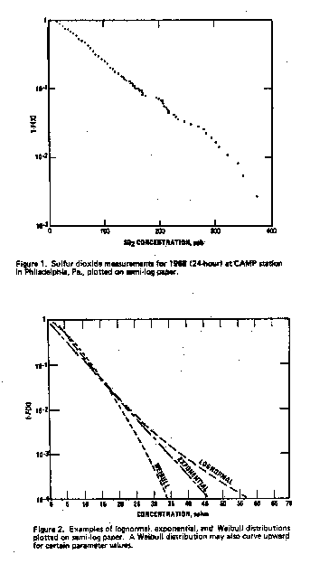
as shown in Figure 1. Figure 1. Sulfur dioxide
measurements for 1968 (24-hour) at CAMP station in Philadelphia,
PA., plotted on semi-log paper. A discussion of this plotting
is contained elsewhere. [5] Figure 2 illustrates how different types
of distributions would appear on such a plot. Figure
2. Examples of lognormal, exponential and Weibull distributions
plotted on semi-log paper. A Weibull distribution may also curve
upward for certain parameter values. The data may also be plotted
on other types of graph paper, such as lognormal or Weibull. The
ideal situation is when the data points lie approximately on a straight
line. The next step is to choose a statistical distribution that
approximately describes the data and to fit the distribution to
the data. This may be done by least squares, maximum likelihood
estimation, or any method that gives a reasonable fit to the top
10% of the data. An obvious question is "what constitutes a reasonable
fit?" This can be judged visually by plotting the fitted distribution
on the same graph as the data points. Because of the intended use
of the distribution, the degree of approximation for the top 10%,
5%, 1% and even .5% of the data must be examined. The most obvious
check is to examine departures of the actual data points from the
fitted distribution. As a general rule there should be no obvious
pattern to the lack of fit in terms of under- or over-prediction,
or trend. For example, if the fitted distribution underestimates
all of the last eight data points by more than 5%, then it must
be established that the fitted distribution is reasonable. Such
an argument might involve showing that the majority of these data
points all occurred in the same period and that the meteorology
for these particular days was extremely unusual. The claim that
this meteorology was unusual would also have to be substantiated
by examining historical meteorological data. It should be noted
that this extra effort is not routinely required and would only
be necessary when the fit appears inadequate. The design value corresponds
to a frequency of 1/365 and in some cases the empirical frequency
distribution function will be plotted in this range. In such cases,
the fitted distribution should be consistent with the empirical
distribution in this range. This can be examined graphically by
locating the concentration on the empirical frequency distribution
function corresponding to a frequency of 1/365. By construction,
there will be measured data points on either since of this value.
The two measured concentrations below this value and the two measured
concentrations above this value will be used as a constraint in
fitting a distribution. If the fitted distribution results in a
design value that differs by more than 5% from all four of these
measured concentrations, some explanation should be presented indicating
the reasons for this discrepancy. It should be noted that in some
cases, there may be only one rather than two measured values on
the empirical frequency distribution with frequencies less than
1/365. In these cases, the upper constraint would consist of one
rather than two data points.
(2) Using the Empirical Frequency Distribution of Several
Years of Data (Graphical Estimation)
It should be noted that if several years of fairly complete data
are available it is not necessary to even fit a statistical distribution.
The concentration value corresponding to a frequency of 1/365 may
be read directly off the graph of the empirical distribution function
and used as the design value.
If the data records are not sufficiently complete, then the empirical
distribution function will not be plotted for the 1/365 frequency
and it will be necessary to fit a distribution to estimate the design
value. However, whenever sufficient data are available, this technique
provides a convenient means of graphically estimating the design
value.
(3) Table Look-up
An obvious point that can initially be overlooked in the discussion
of these techniques is that the final choice of a design value is
primarily influenced by the few highest values in the data set.
With this in mind, it is possible to construct a simple table look-up
procedure to determine a design value. Again, it is important to
treat the number of values properly to ensure that the data adequately
reflects all portions of the year.
To use this tabular approach it is only necessary to know the
total number of daily values, and then determine a few of the highest
data values. For example, if there are 1,017 daily values then the
ranks of the lower and upper bounds obtained from Table 1 are 3
and 2. This means that an appropriate design value would be between
the third highest and second highest observed values. In using this
table the higher of the two concentrations may be used as the design
value. Therefore, in this particular case, it suffices to know the
three highest measured values during the time period.
TABLE 1

TABULAR ESTIMATION OF DESIGN VALUE
-----------------------------------------------------------
Number of    Rank of      Rank of        Data Point Use for
Daily Values Upper Bound  Lower Bound     Design Value

365 to 729        1          2            highest value

730 to 1094       2          3            second highest

1095 to 1459      3          4            third highest

1460 to 1824      4          5            fourth highest

1825 to 2189      5          6            fifth highest
-----------------------------------------------------------
This look-up procedure is basically a tabular technique for determining
what point on the empirical frequency distribution corresponds to
a frequency of 1/365. By construction, the table look-up procedure
overestimates the design value. For instance, in the example with
1,017 values, an acceptable design value would lie closer to the
lower bound. This could be handled by interpolation between the
second and third highest values. However, rather than introduce
interpolation formulas it would be simpler to merely use the previously
discussed graphical procedure.
For the cases that are 75% complete but still have less than 365
days, the maximum observed concentration may be used as a tentative
design value as long as the data set was 75% complete during the
peak times of the year. In this case it must be recognized that
the design value is quite likely to require future revision. In
principle, if statistical independence applied, this maximum observed
concentration would equal or exceed the 1/365 concentration about
half the time. However, the failure to adequately account for yearly
variations in meteorology makes any estimate based on a single year
of data very tentative.
(4) Fitting a Separate Distribution for Each Year of Data
(Conditional Probability Approach)
The previous method required grouping data from several years
into a single frequency distribution. In some cases data processing
constraints may make this cumbersome. Therefore, an alternate approach
may be used that allows each year to be treated individually. In
considering this alternate approach it is useful to briefly indicate
the underlying framework. This particular approach uses conditional
probabilities and in most cases it would probably be more convenient
to use one of the previous methods. However, the underlying framework
of this method has sufficient flexibility to warrant its inclusion.
Suppose that the air quality data at a particular site may be
approximated by some statistical distribution F (x|T), where T (theta)
denotes the fitted parameters. Suppose further, that the values
of the fitted parameters differ from year to year, but that the
data may still be approximated by the same type of distribution.
Intuitively that would mean that while the same type of distribution
describes each year of data, the values of the parameters would
change from year to year reflecting the prevailing meteorology for
the year. In theory it could be possible to define a set of meteorological
classes, say m(i), so that the distribution function of the air
quality data could be defined for each one of these meteorological
classes. Then for each meteorological class, m (i), there would
be an associated air quality distribution function denoted as F[x|m(i)],
the distribution function for x given the meteorological class m
(i). Using the standard rules of conditional probability the distribution
function F(x) may be written as:
	F(x) = SUM from i   {F [ x|m (i) ] }   P[ m (i) ]
                       (SUM represents the Greek sign for sigma)

where P [m (i) ] is the probability of meteorological class m (i) occurring.

	Continuing this approach the expected number of exceedances may be written as:

	E (e) =SUM from i    P [ x > s| m (i) ] * P [ m (i) ]

where s denotes the standard level.
Initially, the above framework may seem to be too theoretical
to have much practical use. However, it will seen in Section 4 that
this approach may afford a convenient means of determining the expected
number of exceedances per year when limited historical data is available.
For the present discussion, it suffices to indicate how this approach
may be used when ambient data sets are available.
Suppose that five years of ambient measurements are available.
An approximating statistical distribution may be determined as discussed
previously for each year, denoted as Fi (x). This would be analogous
to the F [x|m (i) ] in the above discussion. Then the distribution
function of F (x) may be written as:
F (x) =SUM from i = 1 to 5 Fi (x) * 1/5
where Fi is analogous to F[x|m (i) ] and P [m (i) ] is assumed
to be 1/5. The design value may then be determined by setting 1-F
(d) = 1/365 and solving for d, the design value. This is equivalent
to determining the concentration d so that:
SUM from i = 1 to 5 [1-Fi (d) ] * 1/5 = 1/365
In general, it may not be possible to explicitly solve this equation
for d, but the answer may be obtained iteratively by first guessing
an appropriate design value.
The use of this equation can perhaps best be illustrated by a
simple example with two years of data. Suppose the data for each
year may be approximated by an exponential distribution although
the parameter is different for the two years. In particular let
F1(x) = 1 - EXP (-43.4x) and
F2(x) = 1 - EXP (-37.6x).
Using the previous equation, the design value d must be determined
so that
1/2 EXP (-43.4d) + 1/2 EXP (-37.6d) = 1/365 or
365 * {1/2 EXP (-43.4d) + 1/2 EXP (-37.6d) } = 1.
If .15 is used as an initial guess for d this equation gives a
value of .92 rather than 1. If .145 is used the resulting value
is 1.12, indicating that the design value is between .145 and .15.
Guessing .148 gives a value of .99, i.e.
365 {1/2 EXP (-43.4 * .148) + 1/2 EXP (-37.6 * .148)} =. 99
This is sufficiently close to 1 and is a reasonable stopping place
in deterring the design value.
3.4 Quick Test for Design Values
All of the approaches in the previous section have one thing in
common; namely, their purpose. Each technique is intended to select
an appropriate design value, i.e., a concentration with expected
number of yearly exceedances equal to 1. With this in mind a quick
check may be made to determine how reasonable the selected design
value is. This may be done by counting the number of observed daily
values that exceed the selected design value and computing the average
number of exceedances per year. For example, if the selected design
value was exceeded 4 times in 3 years, then the average number of
exceedances per year is 1.2. Ideally, this average should be less
than or equal to 1, but for a variety of reasons, somewhat higher
values may occur. However, if this average is greater than 2.0,
the design value is questionable. In such cases, the design value
should either be changed, or, if not changed, careful examination
should be performed to substantiate this choice of a design value.
3.5 Discussion of Data Requirements
The use of the previous approaches presupposes the existence of
an adequate data base. Both approaches were presented in the context
of having several years of ambient data. In many practical cases
the available data base may not be so extensive. Although these
statistical approaches may be used with less data, some caution
is still required to ensure a minimally acceptable data set. In
general, statistical procedures permit inferences to be made from
limited data sets. Nevertheless, the initial data set must be representative.
For example, if no data is available from the peak season, then
any extrapolations would require more than merely statistical procedures.
Therefore, the input data sets should be at least 50% complete for
the peak season with no systematic pattern of missing potential
peak hours. This 50% completeness criterion should be viewed in
the context of the type of monitoring performed. A continuous monitor
that fails to produce data sets meeting this criteria has in effect
a down-time of more than 50%. With such a high percentage of down-time
for the instrument even the recorded values should be viewed with
caution.
In employing approaches that group data from all years into one
frequency distribution, it should be verified that all years have
approximately the same pattern of missing values. Furthermore, if
the number of measurements during the oxidant season differs by
more than 20% from one year to another, then the conditional probability
approach should be used. The reason for this constraint is to ensure
that variations in sample sizes do not result in disproportionate
weighting of data from different years.
Another point of concern is how many years of data should be used.
Intuitively, it would be reasonable to use as many years of data
as possible as long as emissions have not changed "appreciably".
Obviously, this suggests that some guidance be provided on what
percent change in emissions is permissible. To some degree any such
specification is arbitrary. However, the more relevant point is
that the specified percentage be reasonable. The reason for a cut-off
is to ensure that the impact of increased emissions is not masked
by the use of air quality data occurring prior to these emission
increases. If an area is in violation of the standard, then emission
changes should be expected as control programs take effect. Also,
the design value serves as a guide to achieving the standard and
is, in a sense, merely the means to an end rather than an end in
itself. Therefore, no more than a 20% variation between the lowest
and highest years is recommended. It should be noted that a total
variation of 20% may translate into a + or - 10% variation around
the average.
If emissions have increased by more than 20%, then additional
years should not be incorporated unless the air quality values can
be adjusted for the change in emissions. For cases in which emissions
have decreased by more than 20%, the earlier data may be used after
adjustment or use without change knowing that the design value will
consequently be conservative. Although this document does not discuss
methods for performing this adjustment, it is useful to mention
the basic principle involved. The selection of a design value inherently
implies the existence of an acceptable model for taking an air quality
value and determining the emission reduction required to reduce
this value to the standard. In principle, then, this same model
may be used in reverse to take the emission change known to have
occurred and use the model to scale the previous data sets. Attempting
to adjust older historical data may initially seem to be an unnecessary
complication but the more data that can be used to estimate the
design value the more likely it is that a proper design value is
selected. Because considerable effort could be expended in revising
a control strategy, this additional effort may be warranted.
3.6 Example Design Value Computations
As in the previous discussion of compliance assessment, it is
convenient to conclude this section with examples illustrating the
main point involved in applying these various techniques. For purposes
of illustration, all four techniques are used on the same data set.
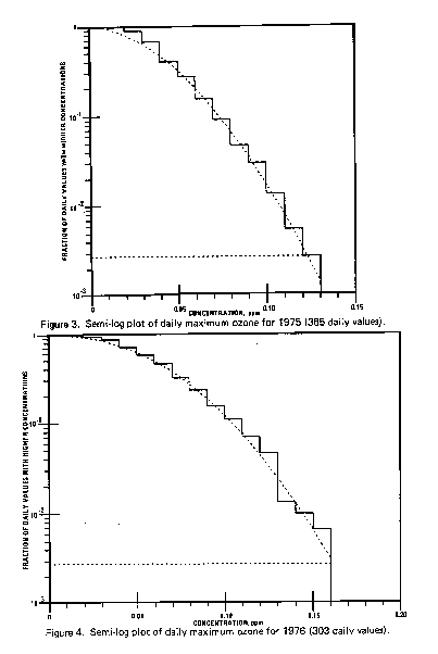
Figures 3, 4 and 5 display semi-log plots of daily ozone values
for 1974, 1975 and 1976 at a sample site. These data are plotted
using previously discussed conventions. [5] The horizontal axis
is concentration (in ppm) and the vertical axis is the fraction
of values exceeding this concentration. A horizontal dotted line
is shown at a frequency of 1/365 and the dotted line represents
a Weibull distribution approximating the data. This particular fit
was done by "eye-balling" the data, but suffices for the purposes
of illustration.
Figure 3. Semi-log plot of daily maximum
ozone for 1975 (365 daily values).
Figure 4. Semi-log plot of daily maximum
ozone for 1975 (303 daily values)
Figure 5. Semi-log plot of daily maximum
ozone for 1977 (349 daily values).
Figure 6 is a similar plot for all three
years of data grouped together. The high and second high values
for the three years are: (.13 and .12), (.16 and .16) and (.15 and
.14).
Method 1: fitting a single distribution to data from all three
years.
The Weibull distribution plotted in figure 6 for the three years
of data is described by the equation:
F(x) = 1 - EXP [-(x/.0609) **2.011 ].
** = raised to a power
Figure 6. Semi-log plot of daily maximum
ozone for three years: 1975, 1976,1977 (1,017 daily values)
Setting F(x) = 1 - 1/365 and solving for x gives .147 which is
the design value because it corresponds to a frequency of exceedance
of 1/365. Using this quick check, there are three values above .147
so the average number of yearly exceedances is 1.
Method 2: Graphical estimation
Referring to Figure 6 it may be seen that the empirical frequency
distribution function crosses the line plotted at 1/365 at a concentration
of .15 and, therefore, this is the design value selected by this
method.
Using the quick check there are only two data values above .15
and, therefore, the average number of yearly exceedances of the
design value is .67 which is acceptable.
Method 3: Table look-up
A total of 1,017 data values were recorded during the three year
period. Using Table 1, this method says that the second highest
value may be used as the design value. Therefore this method yields
.16 as the design value. The quick check gives 0 as the average
number of yearly exceedances of the design value although there
are two values exactly equal to this estimated design value. As
indicated earlier, this procedure is somewhat conservative in that
it tends to overestimate the design value.
Method 4: Conditional probabilities
Separate two parameter Weibull distributions were fitted to each
yearly data set as shown in the groups. Using the form of equation
5 gives the equation:
1/365 = 1/3 EXP {-(d/.0467)**1.835 } + 1/3 EXP {-(d/.0705)**2.139
} + 1/3 EXP {-(d/.0629)**2.180}
Solving for d (by successive guesses) gives .15 as the design
value. Using the quick check gives two values above the design value
and therefore an average yearly exceedance rate of 2/3.
4. APPLICATION WITH LIMITED AMBIENT DATA
Virtually all of this discussion has focused upon the use of ambient
data. Historically, air quality models have been quite useful in
providing estimates of air quality levels in the absence of ambient
data. The proposed wording of the standard does not preclude the
use of such models. As models that provide frequency distributions
of air quality are developed, their use with the proposed standard
will be convenient.
Another potential means of estimating air quality data involves
the use of conditional probabilities. While the use of conditional
probabilities was discussed earlier in terms of combining different
years of data, a more promising use of this technique would involve
the construction of historical air quality data sets from relatively
short monitoring studies. Very limited ambient data or air quality
models may be used to develop frequency distributions for certain
types of days or meteorological conditions. Then past historical
meteorological data may be used to determine the frequency of occurrence
associated with these meteorological conditions. This information
may then be combined using conditional probabilities to obtain a
general air quality distribution. This particular approach could
even be expanded to allow for changes in emissions.
No matter what approach is chosen the two quantities of interest
are : (1) the expected number of exceedances per year and (2) the
design value, i.e., that concentration with expected number of years
exceedances equal to 1. However, these modeling and conditional
probability constructions may make it possible to assess the risk
of violating the standard in the future based upon limited historical
data.
5. REFERENCES
1. 40CFR50.9
2. Fed., Reg., 36 (84):8186 (April 30, 1971)
3. "Guidelines for Interpretation of Air Quality Standards," Office
of Air Quality Planning and Standards. Publ. 1.2-008 US Environmental
Protection Agency, RTP, NC. February 1977.
4. Larsen, R. I. A Mathematical Model for Relating Air Quality
Measurements to Air Quality Standards. US Environmental Protection
Agency, RTP, NC. Publ. AP-89, 1971.
5. Curran, T.C. and Frank , N.H. Assessing the Validity of the
Lognormal Model When Predicting Maximum Air Pollutant Concentrations.
Paper No. 75-51.3, 68th Annual Meeting of the Air Pollution Control
Association, Boston, MA. 1975.
6. Mage, D. T. And Ott, W.R. An Improved Statistical Model for
Analyzing Air Pollution Concentration Data. Paper No. 75-51.4, 68th
Annual Meeting of the Air Pollution Control Association, Boston,
MA. 1975.
7. Johnson, T. A Comparison of the Two-Parameter Weibull and Lognormal
Distributions Fitted to Ambient Ozone Data, Quality Assurance in
Air ollution Measurement Conference. New Orleans, LA. March 1979.
8. Breiman, L., et al. Statistical Analysis and Interpretation
of Peak Air Pollution Measurements Technology Service Corporation,
Santa Monica, CA. 1978.
|