Marietta Echeverria, R. David Jones, Chuck Peck, Mohammed Ruhman, Andrew Shelby, Shelly Thawley, Nelson Thurman

Office of Pesticide Programs
Environmental Protection Agency
March 16, 2012

On this Page

• Memorandum

1. Summary
2. Purpose and History
3. Development of Revised and New PCA Adjustment Factors
   • National PCA Adjustment Factors
     • PCA Adjustment Factors for Major Crops and Crop Groups
     • Adjustment Factors for Turf
     • PCA Adjustment Factors for Combined Crops
   • Regional All Agriculture PCA Adjustment Factors
   • Regional Crop Group PCA Adjustment Factors
4. Quality Assurance and Quality Control
   1. Confirmation of PCA Adjustment Factors
   2. Comparison to Monitoring Data
      • Methodology
      • Results
      • Conclusions
   3. Comparison to Aerial Photography
5. Guidance for Use
   • National Scale Assessments
   • Use on Rice
   • Regional Refinements
6. Reporting Results
7. Future Refinements
8. Literature Cited

• Appendix A Monitoring vs. Modeling Comparison
• Appendix B WQTT Advisory Memorandum
• Appendix C Confirmation of PCA Adjustment Factors
• Appendix D GIS Processing Steps for HUC 8 Watershed PCAs

Tables

• Table 1 Recommended national percent cropped area (PCA) adjustment factors
• Table 2 Recommended regional percent cropped area (PCA) adjustment factors for all agricultural crops for use in refined drinking water assessments
• Table 3 Maximum percent cropped area (PCA) adjustment factor for each HUC size based on crop or crop group
• Table 4 Regional maximum percent turf area adjustment factors
• Table 5 Maximum percent cropped area (PCA) adjustment factor for crop combinations
• Table 6 Maximum percent cropped area (PCA) adjustment factors for each region
• Table 7 Region specific crop group PCA adjustment factors
• Table 8 Example table for reporting EDWCs in drinking water exposure assessments

Figures

• Figure 1 National hydrologic unit classification system
• Figure 2 Major regions (HUC-2) represented by regional PCA adjustment factors overlain with U.S. state boundaries
• Figure 3 All agriculture PCA by 8-digit HUCs
• Figure 4 Decision tree for national PCA adjustment factor determination

---

Memorandum

March 16, 2012

SUBJECT: Guidance on Development and Use of Percent Cropped Area and Percent Turf Area Adjustment Factors in Drinking Water Exposure Assessments: 2012 Update

FROM: Donald Brady /s/, Director, Environmental Fate and Effects Division (7507P), Office of Pesticide Programs

TO: Environmental Fate and Effects Division (7507P), Office of Pesticide Programs

Through this memorandum I am announcing the guidance entitled "Development and Use of Percent Cropped Area and Percent Turf Area Adjustment Factors in Drinking Water Exposure Assessments: 2012 Update". The revised document is dated March 16, 2012 and supersedes the guidance entitled "Development and Use of Percent Cropped Area Adjustment Factors in Drinking Water Exposure Assessments" dated September 9, 2010. The new guidance will be made available on the Models for Pesticide Risk Assessment webpage. The new guidance adds a turf adjustment factor and percent cropped area (PCA) adjustment factors for vegetables and orchard/vineyard. Additionally, existing PCA adjustment factors have been updated with the recent Agricultural Census (2007) and National Land Cover Data (2006).

In general, any drinking water modeling for surface water that begins on or after the week of March 19,2012 should be conducted after review and consistent with "Development and Use of Percent Cropped Area and Percent Turf Area Adjustment Factors in Drinking Water Exposure Assessments: 2012 Update" document dated March 16,2012.

Top of Page

---

Development and Use of Percent Cropped Area and Percent Turf Area Adjustment Factors in Drinking Water Exposure Assessments: 2012 Update

1. Summary

   This guidance document updates the Office of Pesticide Programs' (OPP's) percent cropped area (PCA) adjustment factors, including the national default, crop specific, crop combinations, and regional adjustment factors. Additionally, turf, vegetable crop group, orchard/vineyard crop group and rice specific adjustment factors are included in this update. Drainage areas with the Hydrologic Unit Code 8 (HUC-8)¹ designation are used to derive these adjustment factors. The instructions for using the PCA adjustment factors and the documentation for how the values were calculated are included in this document. Other changes include a clarification and expansion of the guidance sections for use and reporting of PCAs. Table 1 lists the recommended PCAs for crops, crop groups and crop combinations to be used in national drinking water assessments. Table 2 lists the recommended regional PCAs for all agricultural crops to be used in refined drinking water assessments.

   ---

   ¹ Hydrologic units are part of a hierarchical system for classifying and mapping the watersheds in the United States (Seaber, et al., 1987). The largest units (regions) are designated by two digits, and hence are often called 2-digit HUCs. Subdivisions of regions are designated with additional digits. There are 2,264 8-digit HUCs in the United States. The Reference 8-digit HUC is the watershed where the maximum PCA occurred.

   ---

   Table 1
   Recommended national percent cropped area (PCA) adjustment factors
   (and information on sub-basins² from which they were derived)

   CROP, Crop Group, or Crop combinations4	MAXIMUM PERCENT CROPPED AREA (as a decimal)	REFERENCE HYDROLOGIC UNIT CODE (8-DIGIT HUC1)	REFERENCE STATE
   Corn	0.61	07080204	Iowa
   Soybeans	0.57	04100011	Ohio
   Wheat	0.38	11030010	Kansas
   Cotton	0.33	12050003	Texas
   Orchard/Vineyard	0.23	18030009	California
   Rice3	0.21	18020104	California
   Vegetable	0.29	18060011	California
   Turf	0.45	04090004	Michigan
   All Agricultural Land (default national)	0.91	09020306	Minnesota
   Non-Agricultural Non-Turf Uses	1.0	(not applicable)	(not applicable)
   Corn-Wheat	0.61	07080204	Iowa
   Soybeans-Wheat	0.70	04100011	Ohio
   Turf-Corn	0.67	07080204	Iowa
   Turf-Orchard/Vineyard	0.45	04090004	Michigan
   Turf-Soybean	0.64	04100011	Ohio
   Turf-Vegetable	0.48	18060011	California
   Turf-Wheat	0.45	04090004	Michigan
   Vegetable-Orchard/Vineyard	0.34	18060011	California
   Turf-All agriculture	0.95	09020306	Minnesota

   1. The Reference HUC and State indicate the location where the maximum PCA was derived.

   2. For this document, OPP has adopted the USGS convention for describing HUCs as regions, sub-regions, basins, sub-basins, watersheds and sub-watersheds (see Hydrologic Unit Maps).

   3. Rice culture violates two assumptions of PCA adjustment factors: that there is uniform hydrology across the drainage area and that chemical concentrations at drinking water intakes are being driven by runoff. Rice paddy hydrology is substantially different from the surrounding drainage area and rice paddy water release does not occur at the same time as runoff events. The rice PCA may only be used in models that account for rice hydrology.

   4. The table does not include crop combinations involving cotton because the combination of cotton and other major crops (corn, soybeans, wheat, turf) does not exceed the maximum PCA factor for the other crop. While the combination of cotton and any of these other crops, will exceed the maximum PCA factor for cotton alone, it does not exceed the maximum PCA factor for the other crop, which occurs outside of the cotton-growing region. Thus, for a national screening assessment that involves pesticide use on cotton and one of the other major crops, the PCA factor for the other crop will provide a protective upper end PCA factor for the combined crops.

   Table 2
   Recommended regional percent cropped area (PCA) adjustment factors for all agricultural crops
   for use in refined drinking water assessments

   Location	Regional Basin	Regional Basin Name	HUC-8 PCA Adjustment Factor	REFERENCE HYDROLOGIC UNIT CODE (8-DIGIT HUC1)	REFERENCE STATE
   East of Eastern Divide	01	New England	0.13	01010005	Maine
   	02	Mid Atlantic	0.34	02080109	Virginia
   	03	South Atlantic-Gulf	0.41	03130010	Georgia
   Mid-Continent (Mississippi River Basin)	04	Great Lakes	0.81	04100008	Ohio
   	05	Ohio	0.81	05120205	Indiana
   	06	Tennessee	0.35	06040006	Kentucky/Tennessee
   	07	Upper Mississippi	0.88	07130002	Illinois
   	08	Lower Mississippi	0.86	08020201	Missouri
   	09	Souris - Red - Rainy	0.91	09020306	Minnesota/ North Dakota
   	10	Missouri	0.87	10270201	Nebraska
   	11	Arkansas - White - Red	0.75	11030003	Kansas
   	12	Texas Gulf	0.69	12050005	Texas/New Mexico
   	13	Rio Grande	0.44	13090002	Texas
   West of Western Divide	14	Upper Colorado	0.13	14080203	Utah/Colorado
   	15	Lower Colorado	0.19	15050303	Arizona
   	16	Great Basin	0.25	16010202	Idaho/Utah
   	17	Pacific Northwest	0.66	17060109	Washington/Idaho
   	18	California	0.61	18030009	California

   Top of Page

   ---

2. Purpose and History

   The purpose of this document is to provide information on the development of the revised and new percent cropped area (PCA) adjustment factors and guidance on their use in estimating the exposure in drinking water derived from vulnerable surface water supplies. Prior to 2000, the Agency assumed the entire area of the watershed was planted with the crop of interest (i.e., 100% crop coverage). In 2000, the Agency implemented the PCA adjustment factor to account for the percentage of the watersheds planted with a crop, recognizing that in many cases a watershed large enough to support a drinking water facility will not be planted completely with a single crop. This step was implemented to improve the quality and accuracy of the Office of Pesticide Programs' (OPP) modeling of drinking water exposure for pesticides. The PCA adjustment factor is used to adjust the model-predicted estimated drinking water concentration (EDWC) of a pesticide where each EDWC is multiplied by the PCA adjustment factor (expressed as a decimal) for the crop(s) of interest.

   This document supersedes all previous PCA guidance documents. Previous PCA documentation includes Applying a Percent Crop Area Adjustment to Tier 2 Surface Water Model Estimates for Pesticide Drinking Water Exposure Assessments, dated December 7, 1999, and Use of Regional Percent Crop Area Factors in Refined Drinking Water Assessments, dated July 25, 2003. These documents were merged in Development and Use of Percent Cropped Area Adjustment Factors in Drinking Water Exposure Assessments, dated September 9, 2010. In the current document, the default all agriculture PCA adjustment factor, the crop specific adjustment factors and region specific adjustment factors are updated to reflect new data. Additionally, turf, all vegetable crop group, orchard/vineyard crop group and rice specific adjustment factors are included.

   The concept of using a factor to adjust the concentrations from modeling to account for land use was first proposed to the Federal Insecticide, Fungicide, and Rodenticide Act (FIFRA) Scientific Advisory Panel (SAP) in December, 1997 (Jones and Abel, 1997). In May 1999, OPP presented a proposed methodology to the SAP: "Proposed Methods for Determining Watershed-derived Percent Crop Areas and Considerations for Applying Crop Area Adjustments to Surface Water Screening Models" (Effland, 1999). In its review, the SAP concluded that "the model appeared to perform reasonably well with major crops in the Midwest and can be comfortably applied under those conditions." The original guidance was based on this proposed methodology, as well as recommendations from the SAP. The SAP (1999) recommended that OPP apply PCA adjustment factors to the modeled concentrations when a pesticide was applied only to one of four major crops (corn, soybeans, wheat, and cotton), or a combination of these crops, given that national coverage was only available at the HUC-8 scale. These maximum PCA adjustment factors represent the potential maximum national percent cropped area and, therefore, are applied no matter where that crop is modeled.

   In September 2000, OPP developed a national "default PCA" adjustment factor to modify exposure estimates for any agricultural crop other than the four "major" crops that the SAP endorsed. The default PCA was not applied for non-agricultural uses of a chemical . In 2011, EFED began the process of updating the PCA adjustment factors using current data sources. These agricultural PCAs were derived using the National Land Cover Dataset (NLCD) (2006) and the National Agriculture Statistics Service (NASS) 2007 Agricultural Census (2010). Using the NLCD (2006), a national spatial coverage of turf was developed by Oak Ridge National Laboratory under a contract from OPP's Environmental Fate and Effects Division (EFED). The turf map was derived using all developed landcover classifications and deducting impervious surfaces. Lastly, the national default PCA adjustment factor was updated in accordance with recent agricultural data and represented the largest amount of land in agricultural production in any HUC-8² watershed³ in the coterminous United States.

   For minor crops, the SAP (1999) found that the use of PCA adjustment factors derived from information on 8-digit HUCs and county-based crop acreages were too coarse for a usable estimate. In their rationale, the SAP stated that most drinking water supplies were fed by smaller watersheds that could have different PCA adjustment factors. PCA adjustment factors developed for 8-digit watersheds versus 10- or 12-digit watersheds are substantially different and result in larger PCAs at progressively smaller watershed scales. In general, the HUC-8 watersheds are larger than 700 square miles in size (Seaber et al., 1987). The SAP concluded that PCA estimates based on the larger 8-digit HUCs may underestimate the percentage of agriculture present in smaller watersheds (SAP, 1999). An EPA analysis in the Organophosphate Cumulative Risk Assessment determined that cropping intensity is variable (i.e., cropping area is not uniformly distributed throughout a county) and found that smaller watersheds capable of supporting drinking water supplies may have PCAs much different from those represented by the 8-digit HUC. An example is the Willamette River Valley, Oregon, where the HUC-8 all agriculture PCA for that valley was less than 30%, yet the USGS reported smaller drainage areas in the valley with up to 99% agriculture (OPP, 2002).

   As such, the SAP found the use of PCA adjustment factors could potentially underestimate exposure estimates for minor crops at the HUC-8 level and advised OPP to further investigate possible sources of error. Though drainage areas delineated at a smaller scale than HUC-8 are now available, this update of the PCAs maintains the HUC-8 scale because OPP anticipates using drinking water specific watersheds for derivation of PCAs in the near future. While some drinking water watersheds will be smaller than respective HUC-8 drainage areas, some will also be larger than HUC-8 drainage areas. OPP is currently working on the next generation of PCAs based on delineated drinking water-specific watersheds.

   The SAP provided only minimal guidance on applying the PCA adjustment factor for multiple crops in a watershed. They recommended that the PCA adjustment factor for multiple crops be based on the single watershed that had the highest percentage of the combination of the crops being modeled, rather than on summing the maximum PCA adjustment factors for the individual crops from different watersheds.

   Because some pesticides may be applied to multiple crops, OPP developed additional PCA adjustment factors that represent the potential combined amount of land that may be in production for these crops. Turf is also included in PCA combinations. When applications include non-agricultural, non-turf pesticide use areas (e.g., rights of way, ornamentals, etc.), no adjustment is made, (i.e. the PCA = 1) as the Geographic Information System (GIS) coverage used to develop the PCA adjustment factors represents only agricultural land and turf sites. Similarly, PCAs are not applicable to areas outside the coterminous United States (e.g., Alaska, Hawaii, and Puerto Rico). The PCA adjustment factors used in national (non-refined) drinking water exposure assessments are presented in Table 1. Besides these national PCA adjustment factors, OPP developed 18 "regional default PCA" adjustment factors that can be used for spatial refinements of exposure (e.g., for estimating exposure in a specific region of the United States), as described below (Table 2). Similar to the national default PCA, these regional default PCA adjustment factors represent the largest amount of land in agricultural production in any 8-digit HUC watershed within a given 2-digit HUC region in the coterminous United States.

   Additional information about how these values were derived can be found in the following sections of this document. Section 3.0 describes the methods used to derive the PCA adjustment factors with the newly derived turf, crop or crop groups PCAs and default PCA at the national and regional scales. Section 4.0 describes the quality assurance and quality control steps that have been taken, and Section 5.0 describes when and how to apply PCA adjustment factors to surface water model estimates. Finally, Section 6.0 discusses reporting results and assumptions and limitations of this methodology and Section 7.0 discusses future refinements.

   ---

   Footnotes

   ² HUC stands for Hydrologic Unit Code. Hydrologic units are part of a hierarchical system for classifying and mapping the watersheds in the United States (Seaber, et al., 1987). The largest units (regions) are designated by two digits, and hence are often called 2-digit HUCs. Subdivisions of regions are designated with additional digits. There are 2,264 8-digit HUCs in the United States. The Reference 8-digit HUC is the watershed where the maximum PCA occurred.

   ³ For this document, OPP has adopted the USGS convention for describing HUCs as regions, subregions, basins, subbasins, watersheds and subwatersheds (see Hydrologic Unit Maps).

   Top of Page

   ---

3. Development of Revised and New PCA Adjustment Factors

   The Environmental Fate and Effects Division (EFED) uses PCA adjustment factors in drinking water exposure assessments to account for the fact that a watershed of sufficient size to supply a drinking water source is not likely to be devoted entirely to growing crops or turf. The PCA adjustment factors are derived by determining the portion of each drainage area (represented by nationally-available 8-digit HUCs) in the continental United States devoted to growing crops, in general, and for certain individual crops, crop groups, and turf.

   Since PCA adjustment factors were initially developed, National Land Cover Dataset (NLCD) and National Agriculture Statistics Survey (NASS) Agricultural Census data have been updated to improve the PCA estimates. Additionally, a national turf map (ORNL, 2008) has been developed allowing estimation of percent turf area. These updates, refinements and new data more accurately reflect current land use patterns and have facilitated the development of new PCA crop groups.

   Drainage areas can be defined at different scales, from large ones, such as the entire drainage area of the Mississippi River, to small ones that drain into a first-order stream. The USGS developed a hierarchical system of classifying these drainage areas by dividing them into smaller and smaller areas called hydrologic units or HUCs (Seaber et al., 1987). The first order of watershed boundaries are the 21 national regions, followed by 221 sub-regions, 378 basins, and 2,264 sub-basins. This guidance recommends the use of PCAs on the sub-basin scale. Previous to 2007, the sub-basin scale, or HUC-8 drainage area, was the finest resolution available on a national scale. National coverage of hydrologic units is now available at the sub-watershed scale (HUC-12). The sub-watershed level is typically 10,000 to 40,000 acres with some as small as 3,000 acres with approximately 160,000 drainage areas delineated nationwide. OPP evaluated the use of HUC-10 watershed and HUC-12 sub-watershed scale to derive PCAs.

   The results are included in this document for comparative purposes. While some drinking water watersheds will be smaller than respective HUC-8 drainage areas, some will also be larger than HUC-8 drainage areas. OPP is currently working on the next generation of PCAs derived from drainage areas specific to surface water drinking water intakes serving Community Water Systems (CWS).

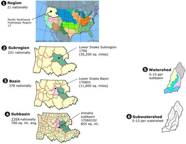   Figure 1
   National hydrologic unit classification system

   Top of Page

   ---

   • National PCA Adjustment Factors

     Development of the national PCA adjustment factors required four principal information sources:

     • The Watershed Boundary Dataset (WBD) HUC8 (version April 21, 2011) and HUC12 (version May 16, 2011) shapefiles (What is the WBD?)

     • Cropland distribution information from the National Land Cover Dataset (NLCD) (2006 National Land Cover Data (NLCD 2006))

     • Census Bureau 1:24,000 scale TIGER file of county boundaries (Census 2000 TIGER/Line(R) Files Technical Documentation).

     • County-level crop information from the 2007 USDA National Agriculture Statistics Service (NASS) Census of Agriculture (specific tables listed in Appendix D) (2007 Census Publications).

     Top of Page

     ---

     • PCA Adjustment Factors for Major Crops and Crop Groups

       A detailed GIS-based methodology of the calculation of adjustment factors is found in Appendix D.

       Development of the all agriculture PCA adjustment factors was based entirely on the NLCD and were calculated as the total area of the row crop class (82) divided by the total area of all classes except open water (11) on a per HUC8 watershed basis. Following this procedure, the default national PCA adjustment factor for agricultural uses was calculated to be 91% for HUC-8 watersheds. This value was based on calculations for HUC 09020306, which is located in Minnesota and is the most heavily cropped 8-digit HUC in the entire United States. The adjustment factor for HUC-10 watersheds is 95% and for HUC-12 watersheds is 100%. The HUC-8 sub-basins are being used for the current recommended PCAs as they were previously approved for use by the FIFRA SAP and can be more rapidly implemented than those based on HUC-10 or HUC-12 watershed boundaries. As watershed boundaries based on current drinking water facility watersheds have been developed and are currently undergoing validation, the extra effort needed to implement HUC-10 or HUC-12 PCA is not warranted as they would not likely be ready by the time the drinking water watershed based PCAs are available.

       Crop-specific PCA adjustment factors for each crop were calculated by blending the NASS county crop statistics with NLCD cropland distributions and summarizing by HUC watershed using the following steps:

       1. Isolate NLCD land cover category 82 (row crops) to create generic cropland distribution map.

       2. Calculate number of agriculture pixels per county.

       3. Combine NASS county-level crop acreage information with row crop pixel information to derive acre per pixel value by crop.

       4. Use acres per pixel per county values to generate derived raster crop-specific maps.

       5. Sum all ag. acres-per-pixel per HUC watershed.

       6. Calculate PCA as crop area divided by total area.

       7. Select the maximum PCA from the distribution.

       The resulting PCAs are presented in the following table.

       Table 3
       Maximum percent cropped area (PCA) adjustment factor for each HUC size based on crop or crop group

       Crop or Crop Group	HUC-8	HUC-10	HUC-12
       Corn	0.61	0.66	0.80
       Cotton	0.33	0.51	0.65
       Orchard/vineyards1	0.23	0.40	0.48
       Rice	0.21	0.36	0.43
       Soybean	0.46	0.54	0.78
       Vegetable2	0.29	0.40	0.64
       Wheat	0.38	0.51	0.59
       All Agriculture3	0.91	0.95	1.00

       1. Orchard/vineyard PCA includes fruit trees, citrus or other groves, vineyards, and nut trees

       2. Vegetable PCA includes artichoke, asparagus, lima bean, snap beans, beets, broccoli, Brussels sprouts, cabbage, cantaloupes, carrots, cauliflower, celery, chicory, collards, cucumbers, daikon, eggplant, escarole/endive, garlic, ginseng, herbs, honeydew, horseradish, kale, lettuce, mustard greens, okra, onions, parsley, peas, peppers, potatoes, pumpkins, radishes, rhubarb, spinach, squash, sweet corn, sweet potatoes, tomatoes, turnips, watercress and watermelons and other vegetables. (REF NASS TABLE 34)

       3. Sod farms are included in "All Agriculture" PCA

       Top of Page

       ---

     • Adjustment Factors for Turf

       Turf uses are a function of both the NLCD developed classes (21 - 24) and row crops (82), the surrogate for sod farms. To account for turf in developed areas, a national turf map was developed by Oak Ridge National Laboratory, under contract with the Environmental Fate and Effects Division (ORNL 2008). The ORNL turf layer is derived from the 2001 NLCD and includes the area classified as developed (classes 21 - 24), minus impervious surfaces. An impervious surface layer is included in the NLCD product. A sod farm map was derived using the blended NASS and NLCD technique used for the other crop-specific adjustment factors. The ORNL turf map was added to the sod farm layer for total area in turf. Turf adjustment factors were then calculated for all HUC8 polygons. A maximum turf value was calculated from the distribution.

       The use of the turf adjustment factor is only appropriate if the chemical of interest is applied to turf only. If any agricultural uses are included, a combination PCA adjustment factor should be used (i.e. 0.95 for national assessments or one of the regional "All Crop-Turf" adjustment factors in Table 7, if appropriate). If the chemical of interest is applied to golf courses only, the turf PCA in conjunction with the "Golf Course Adjustment Factors" is appropriate, refer to Golf Course Adjustment Factors for Simulated Aquatic Exposure Concentrations (OPP, 2005).

       Table 4
       Regional maximum percent turf area adjustment factors

       Regional Basin (HUC-2)	PCA Adjustment Factor	REFERENCE HYDROLOGIC UNIT CODE (HUC-8)	REFERENCE STATE
       1	0.24	01100004	Connecticut
       2	0.39	02030102	New York/Connecticut
       3	0.31	03100201	Florida
       4	0.45	04090004	Michigan
       5	0.22	05010009	Pennsylvania
       6	0.14	06010207	Tennessee
       7	0.42	07120003	Illinois/Indiana
       8	0.35	08010211	Tennessee/Mississippi
       9	0.09	09020104	Minnesota/North Dakota
       10	0.15	10230006	Nebraska/Iowa
       11	0.12	11110101	Oklahoma
       12	0.34	12040104	Texas
       13	0.05	13090001	Texas
       14	0.02	14080202	Colorado/Utah
       15	0.15	15060106	Arizona
       16	0.15	16020204	Utah
       17	0.29	17110012	Washington
       18	0.40	18020111	California

       Top of Page

       ---

     • PCA Adjustment Factors for Combined Crops

       For major crop combinations (e.g., corn and soybeans, corn and wheat, corn and cotton, etc.), similar procedures as described above were applied to develop the PCA adjustment factors.

       1. Follow steps 1 through 6 from methods for PCA Adjustment Factors for Major Crops and Crop Groups.

       2. Add desired crop groups together across each HUC resulting in combination PCA adjustment factors.

       3. Sort resulting combined PCA adjustment factors by size to determine largest combined PCA adjustment factor.

       The PCA adjustment factors for the major crop combinations are listed in Table 5.

       Table 5. Maxiumum percent cropped area (PCA) adjustment factor for crop combinations

       CROP COMBINATIONS	MAXIMUM PERCENT CROPPED AREA (as a decimal)	REFERENCE HYDROLOGIC UNIT CODE (8-DIGIT HUC)	REFERENCE STATE
       Corn-Wheat	0.61	07080204	Iowa
       Soybeans-Wheat	0.70	04100011	Ohio
       Turf-Corn	0.67	07080204	Iowa
       Turf-Orchard/Vineyard	0.45	04090004	Michigan
       Turf-Soybean	0.64	04100011	Ohio
       Turf-Vegetable	0.48	18060011	California
       Turf-Wheat	0.45	04090004	Michigan
       Vegetable-Orchard/Vineyard	0.34	18060011	California
       Turf-All agriculture	0.95	09020306	Minnesota

     In a number of instances, the combination of cotton and another major crop does not exceed the maximum PCA factor for the other crop. This is the case with corn, soybeans, wheat, and turf. While the combination of cotton and any of these other crops, will exceed the maximum PCA factor for cotton alone, it does not exceed the maximum PCA factor for the other crop, which occurs outside of the cotton-growing region. Thus, for a national screening assessment that involves pesticide use on cotton and one of the other major crops, the PCA factor for the other crop will provide a protective upper end PCA factor for the combined crops. Differences between the maximum individual crop PCAs and the combined crop PCAs are likely to become evident in regions where both crops coincide.

     Top of Page

     ---

   • Regional All Agriculture PCA Adjustment Factors

     The default regional PCA adjustment factors represent the HUC-8 watersheds that are the most intensely cropped in each major region of the coterminous United States. The regions are the largest hydrologic units defined by the USGS. They are represented by 2-digit HUCs and divide the United States into 21 major hydrologic areas based on surface topography, eighteen of which cover the coterminous United States. These geographic areas "contain either the drainage area of a major river, such as the Missouri region, or the combined drainage areas of a series of rivers, such as the Texas-Gulf region, which includes a number of rivers draining into the Gulf of Mexico" (Seaber, et al., 1987). The natural hydrologic boundaries of these regions extend into Canada and Mexico, but the regions themselves are truncated at the borders for mapping purposes.

     Because PCA adjustment factors were developed for 8-digit HUCs, which are subdivisions of the major regions (HUC-2), the regional scale was a logical basis upon which to aggregate regional PCA adjustment factors. Figure 2 overlays the HUC-2 region boundaries with U.S. state boundaries. Figure 3 shows all agriculture PCAs for all HUC-8 watersheds.

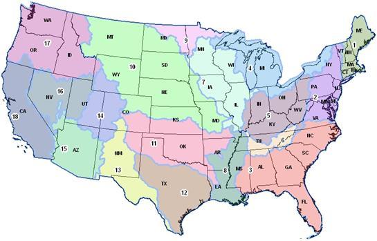     Figure 2
     Major regions (HUC-2) represented by regional PCA adjustment factors
     overlain with U.S. state boundaries

     ---

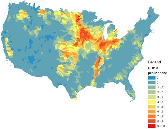     Figure 3
     All agriculture PCA by 8-digit HUCs
     (See Table 2 for the legend for regional basin numbers)

     ---

     To determine the regional PCA adjustment factors, OPP used the same methodology and rationale as was used to identify the national default PCA adjustment factor except the methods were applied for each of the HUC 2 regions. The largest HUC-8-scale PCA adjustment factor within each major region was selected to represent the default PCA adjustment factor for that region. Like the national default PCA adjustment factor, the regional default PCA adjustment factors represent all agriculture, not individual crops. These values can be used as a refinement of drinking water exposure for specific regions of the country for crops other than the major crops, as defined above. Table 6 shows the maximum default agricultural land PCA adjustment factors for each of the 18 major regional basins.

     Table 6
     Maximum percent cropped area (PCA) adjustment factors for each region

     Location	Regional Basin	Regional Basin Name	HUC-8 PCA Adjustment Factor	Reference HUC
     East of Eastern Divide	01	New England	0.13	01010005
     	02	Mid Atlantic	0.34	02080109
     	03	South Atlantic - Gulf	0.41	03130010
     Mid-Continent (Mississippi River Basin)	04	Great Lakes	0.81	04100008
     	05	Ohio	0.81	05120205
     	06	Tennessee	0.35	06040006
     	07	Upper Mississippi	0.88	07130002
     	08	Lower Mississippi	0.86	08020201
     	09	Souris - Red - Rainy	0.91	09020306
     	10	Missouri	0.87	10270201
     	11	Arkansas - White - Red	0.75	11030003
     	12	Texas Gulf	0.69	12050005
     	13	Rio Grande	0.44	13090002
     West of Western Divide	14	Upper Colorado	0.13	14080203
     	15	Lower Colorado	0.19	15050303
     	16	Great Basin	0.25	16010202
     	17	Pacific Northwest	0.66	17060109
     	18	California	0.61	18030009

     Top of Page

     ---

   • Regional Crop Group PCA Adjustment Factors

     Regional PCA adjustment factors for specific crop groups may be used in drinking water assessments provided it is appropriate. These adjustment factors can only be used in limited circumstances in which the chemical's use pattern in a given HUC-2 region is fully characterized by the given crop group. If any other labeled use of the chemical is possible in any part of the HUC-2 region, the regional adjustment factor is not appropriate. For instance, if a chemical is registered only for use on cotton in Texas and wheat in Oklahoma, a region and crop specific PCA adjustment factor cannot be used. HUC-2 11 includes both Texas and Oklahoma; therefore, HUC-8 watersheds on the border may include cotton and wheat crops. In this instance, the most appropriate PCA adjustment factor to apply would be the wheat PCA of 0.38 which is protective for uses including cotton. The following table lists region specific crop group PCA adjustment factors.

     Table 7
     Region specific crop group PCA adjustment factors

     HUC-2	Corn	Cotton	Orchard/Vineyard	Rice	Soybean	Vegetable	Wheat	Turf	All agriculture	All agriculture-Turf
     01	0.02	0.00	0.00	0.00	0.00	0.03	0.00	0.24	0.13	0.24
     02	0.20	0.02	0.01	0.00	0.14	0.03	0.06	0.39	0.34	0.39
     03	0.09	0.14	0.15	0.00	0.13	0.07	0.04	0.31	0.41	0.51
     04	0.31	0.00	0.04	0.00	0.38	0.05	0.11	0.45	0.81	0.89
     05	0.46	0.00	0.02	0.00	0.34	0.01	0.08	0.22	0.81	0.88
     06	0.14	0.05	0.01	0.00	0.11	0.00	0.03	0.14	0.35	0.42
     07	0.61	0.00	0.00	0.00	0.35	0.04	0.12	0.42	0.88	0.94
     08	0.30	0.23	0.00	0.19	0.46	0.01	0.15	0.35	0.86	0.91
     09	0.37	0.00	0.00	0.00	0.34	0.03	0.33	0.09	0.91	0.95
     10	0.56	0.00	0.01	0.00	0.34	0.00	0.34	0.15	0.87	0.91
     11	0.19	0.10	0.02	0.18	0.25	0.01	0.38	0.12	0.75	0.78
     12	0.14	0.33	0.01	0.04	0.01	0.02	0.18	0.34	0.69	0.74
     13	0.03	0.03	0.02	0.00	0.00	0.03	0.04	0.05	0.44	0.49
     14	0.02	0.00	0.00	0.00	0.00	0.00	0.05	0.02	0.13	0.15
     15	0.01	0.05	0.02	0.00	0.00	0.09	0.04	0.15	0.19	0.24
     16	0.01	0.00	0.01	0.00	0.00	0.00	0.06	0.15	0.25	0.28
     17	0.09	0.00	0.05	0.00	0.00	0.06	0.29	0.29	0.66	0.69
     18	0.08	0.07	0.23	0.21	0.00	0.29	0.06	0.40	0.61	0.69

   Top of Page

   ---

4. Quality Assurance and Quality Control

   1. Confirmation of PCA Adjustment Factors

      Part of the quality control (QC) process for the new PCAs was to validate the GIS methods by reprocessing the data and confirming PCA results. The results of this effort are attached in Appendix C.

      Top of Page

      ---

   2. Comparison to Monitoring Data

      As part of the evaluation process for the new PCAs, the model concentrations were compared to monitoring data after the PCAs were applied. The objective of the evaluation was to ensure that the use of PCAs, in conjunction with OPP's typical modeling approach, resulted in concentrations that were protective of vulnerable drinking water watersheds. This section describes the methodology and the results of the evaluation.

      • Methodology

        For the modeling part of the evaluation effort, EFED identified three active ingredients used primarily for each of the eight crop/crop groups for which PCAs were being developed (e.g., corn, cotton, soybeans, wheat, turf, vegetables, orchards, and all crops). Each of the active ingredients was identified as being used primarily on the particular crop or crop group. EFED initially used the USGS NAWQA 2002 maps to identify the prospective pesticides. Then EFED requested use data from OPP's Biological and Economic Analysis Division (BEAD) to determine the extent to which the active ingredients selected were used on the respective crops. After refining the list, EFED collected the physical/chemical properties, fate data, and application information (e.g., application method and maximum single rates, the minimum retreatment interval, date of first application, and maximum number of applications/year) for the active ingredients from the most recent drinking water or endangered species assessment. Using this data, EFED ran Tier II PRZM/EXAMS with PE 5 shell for the standard crops using the index reservoir to estimate the upper 1-in-10 year peak, annual average, and 30-year annual average concentrations. Finally, these values were multiplied by the new HUC 8 and HUC 10 PCAs to develop estimated drinking water concentrations (EDWCs).

        For the monitoring part of the evaluation effort, EFED used USGS monitoring data from community water systems presented in Concentration Data for Anthropogenic Organic Compounds in Ground Water, Surface Water, and Finished Water of Selected Community Water Systems in the United States, 2002-05, USGS NAWQA surface water data (NAWQA Data Export), the USDA's Pesticide Data Program (PDP), the California Department of Pesticide Regulation's Surface Water database (Exit Surface Water Protection Program Database), and data obtained from crop-specific monitoring studies submitted to EPA. CDPR surface water data resulting from spills were excluded from the analyses.

        Using these data sources, EFED determined the highest measured concentration for comparison to the EDWCs. Then EFED compared the PCA-adjusted modeled EDWCs with available monitoring data to evaluate whether the EDWCs would be more protective than monitoring data. Non-targeted monitoring results are not expected to provide maximum estimates as the data are not targeted to pesticide use, and sampling frequency is not adequate to capture peak concentrations. In general, as sampling frequency increases, the peak concentration measured from environmental monitoring increases (SAP 2010). However, if the PCA adjusted values are higher than the monitoring value, there is more confidence that Tier 2 modeling using PCAs will not underestimate drinking water exposure.

        Top of Page

        ---

      • Results

        A comparison of PCA-adjusted EDWCs to the monitoring data as well as the PE5 output files for the various runs is provided in Appendix A. These output files contain the pertinent fate and application data used to estimate the environmental concentrations.

        HUC 8 and HUC 10 PCA adjusted 1-in-10 year peak, annual average, and 30-year average EDWCs were compared with available monitoring data. The results of this comparison are as follows:

        1. HUC 8 and HUC 10 PCA-adjusted peak EDWCs are higher than the monitoring results (2-2,200x) for all chemicals except for atrazine. However, only one atrazine monitoring data point was exceeded.

        2. HUC 8 and HUC 10 PCA-adjusted 1-in-10-year annual mean EDWCs are higher (1.1-315x) than the monitoring concentrations, except for acetochlor, atrazine, cypermethrin, dicrotovos, linuron (HUC 8), phosmet, picloram, and triallate. It should be noted that EDWCs for these chemicals are within an order of magnitude of the monitoring concentrations for all of these chemicals except for atrazine and phosmet.

        3. HUC 8 and HUC 10 PCA-adjusted 30-year average EDWCs values are higher (1.5-315x) than monitoring concentrations except for acetochlor, atrazine, bromoxynil, cypermethrin, dicrotovos, fipronil, linuron, phosmet, picloram, and triallate. It should be noted that these values were the same order of magnitude as the monitoring estimates for all of these chemicals except for atrazine, dicrotofos, and phosmet.

        Top of Page

        ---

      • Conclusions

        In most cases, modeled values adjusted using the newly derived HUC 8 and HUC 10 PCAs were protective estimates, higher than most of the maximum monitoring concentrations. It should be noted that most of the monitoring concentrations used in this comparison were not part of targeted monitoring studies (e.g., there was no correlation between the measured concentrations and any application of the active ingredient). In addition, modeling results are for ten-year return frequencies, while most monitoring data for most sites is collected for a single year. Modeling sites represent a few highly vulnerable sites, while monitoring used in these comparisons represents a large number of sites with a wide range of vulnerabilities to pesticide contamination. This analysis supports the expectation that the results of simulations adjusted with the updated PCAs are protective of human health. However, because the measurement endpoints for the modeling results and monitoring data are not the same, a direct comparison is not appropriate.

      Top of Page

      ---

   3. Comparison to Aerial Photography

      For each PCA adjustment factor reported in this guidance, the corresponding HUC-8 was visually compared to aerial photography of the catchment area. The goal of this quality check was to ensure that erroneous spatial features were not included as part of the cropped or turf area and to verify PCA adjustment factor estimates resemble aerial photography.

   Top of Page

   ---

5. Guidance for Use

   • National Scale Assessments

     For a national-scale drinking water exposure assessment using the index reservoir scenario, surface water source estimated pesticide concentrations (peak and long-term average) should be adjusted (reduced) by the relevant PCA. This adjustment is accomplished by post-processing the modeled values.

     Note that there is an entry for "All Agricultural Land" in Appendix A. This is a default value to use for crops without a specific PCA adjustment factor (e.g., crops other than corn, soybeans, wheat, cotton, vegetables, orchards, rice, and turf). This default value is also used when a pesticide is applied to multiple crops, which may include but are not limited to corn, soybeans, wheat, cotton, vegetables, orchards, and turf. The PCA adjustment factor represents the largest amount of land in agricultural production in any 8-digit HUC unit in the coterminous United States. PCA adjustment factors are not applicable for non-agricultural or non-turf uses (e.g., rights of way, ornamentals, etc.) as data for these uses were not available and therefore were not used to develop PCA adjustment factors. Similarly, PCA adjustment factors are not applicable to areas outside the coterminous United States (e.g., Alaska, Hawaii, and Puerto Rico).

     Selection of PCA adjustment factors depends on the degree of refinement of the exposure assessment and on the crops modeled. Regarding crops, estimates may be developed for the following situations:

     1. a single crop without a crop-specific PCA adjustment factor or multiple crops that are not limited to crops with specific combination crop PCA adjustment factors;

     2. a single crop that has a crop-specific PCA adjustment factor; and

     3. multiple crops that all have crop-specific PCA adjustment factors.

     A decision tree for this process is provided in Figure 4. A discussion of these three situations is provided below.

     Figure 4
     Decision tree for national PCA adjustment factor determination
     ¹ If ai is used for non-agricultural purposes (e.g., rights of way, ornamental, etc.), the national default PCA adjustment factor is 1.0. Otherwise, the national default PCA adjustment factor is 0.91

     ---

     1. If the pesticide is applied to a single crop without a crop-specific PCA adjustment factor, multiply the unadjusted estimated drinking water concentrations (EDWC) for the crop by the national default PCA adjustment factor to obtain the final EDWCs. If the pesticide is applied to multiple crops that are not limited to only corn, soybeans, wheat, cotton, vegetable, orchard, and turf, multiply EDWCs by the national default PCA adjustment factor to obtain the final EDWCs. If the pesticide is used for non-agricultural purposes other than turf (e.g., rights of way, ornamentals, etc.), the national default PCA adjustment factor is 1.0; otherwise, the national default PCA adjustment factor is 0.91.

     2. If the pesticide is only registered for use on a single crop with a developed crop-specific PCA adjustment factor (corn, soybeans, wheat, cotton, vegetable, orchard, or turf), multiply the unadjusted EDWCs by the appropriate PCA adjustment factor for that crop to obtain the final EDWCs. For Tier 2 modeling, the PCA adjustment factor should be applied regardless of where the modeled scenario is located, since the PCA adjustment factor represents the maximum national percent cropped area for that particular crop. As an example, for a pesticide used only on corn, the PRZM/EXAMS EDWCs should be multiplied by 0.61, regardless of the location of the PRZM/EXAMS corn scenario used in modeling. Additionally, the PCA adjustment factor should be applied for individual crops within crop groups. If, for example, the only use for a pesticide is broccoli, the PRZM/EXAMS EDWCs should be multiplied by vegetables PCA adjustment factor (0.29).

     3. If the pesticide is registered only for use on multiple crops for which crop-specific combination PCA adjustment factors have been developed (corn, soybeans, wheat, cotton, vegetable, orchard, turf or rice), multiply all of the unadjusted EDWCs by the PCA adjustment factor for the crop combination to obtain the final EDWCs. The PCA adjustment factor that should be used represents the maximum potential percentage of the watershed that could be planted with these crops. If, for example, a pesticide is only used on corn, then the assumption that no more than 61% of the watershed (at the current HUC scale used) would be planted with corn is likely to hold true. However, if the pesticide is used on both corn and turf, then this assumption no longer holds true, since watersheds often contain both crops with a PCA representing up to 67%. In this case, the model estimates for this use should be re-adjusted to reflect the combined PCA of 67%. If the chemical use pattern includes crops not included for the calculation of PCAs, then all agriculture PCA adjustment factors should be used (Table 1).

     As a refinement, PCA adjustment factors can be applied to the fulltime-series generated by PRZM/EXAMS in a Tier 2 assessment in order to further refine the dietary assessment. The Water Quality Technology Team (WQTT) Advisory "Guidance on Generating Drinking Water Distribution Files for HED's Dietary Risk Assessments" provides instructions for preparing PCA-adjusted EDWC distributions for input into probabilistic dietary models (see Appendix B).

     Top of Page

     ---

   • Use on Rice

     Unlike other PCA adjustment factors, rice cultivation involves manipulation of local hydrology. The use of PCA adjustment factors assumes consistent hydrology throughout a watershed such that all parts of the watershed contribute equally to runoff and runoff occurs contemporaneously with rainfall events. Rice cultivation violates this assumption because rice paddies hold more water than contained in the greater watershed, and water releases are inconsistent with rainfall events. Current EFED models do not account for rice hydrology and rice PCAs are provided only for informational purposes at this time.

     Top of Page

     ---

   • Regional Refinements

     If dietary risks are exceeded in the national scale assessment, the risk manager may ask EFED to refine the pesticide exposure assessment. The risk assessor can either refine the assessment qualitatively by providing additional characterization of potential exposure, or quantitatively by simulating additional sites for each crop, or by using regional PCA adjustment factors in the estimation of the EDWCs. The most appropriate use of regional PCA adjustment factors can be best determined in discussions between risk assessors and risk managers. Possible options that can be considered include the following:

     • Use regional default PCA adjustment factors to refine EDWCs for uses with limited regional extent, such as Section 18 emergency exemptions, Section 24(c) Special Local Need requests, or crops with limited, well-defined growing regions (e.g., citrus).

     • Use regional PCA adjustment factors to better distinguish which crop-chemical scenarios in a pesticide use area may result in the highest surface-water EDWCs. For instance, a crop with a small percentage of total usage of the pesticide grown in the South Atlantic-Gulf basin may have a maximum use rate much higher than the predominant usage on corn in the Midwest. However, after application of the regional PCA adjustment factor to the minor use scenario, the EDWC from the Midwest corn scenario might be higher and, therefore, the driver of the drinking water exposure assessment.

     • Use regional PCA adjustment factors in association with a pesticide usage map to distinguish between the magnitudes of possible exposures for the same crop in different regions of the country and to focus spatial modeling refinements. For instance, EDWCs from a Maine potato scenario may be greater than those from an Idaho potato scenario if the same national PCA adjustment factor is applied to both. However, applying the regional default PCA adjustment factors (12% for Maine and 66% for Idaho) may lead the risk assessor and risk manager to focus on the use in Idaho. This in turn may help risk managers focus mitigation actions on regions where the greatest exposure is likely to occur.

     • Use regional PCA adjustment factors to populate a matrix of regional peak or chronic EDWCs for each labeled use of a pesticide that is expected to result in dietary risk exceedances in order to refine a drinking water exposure assessment. Begin by tabulating states by HUC-2 region where labeled crops are grown and geographically allowed for use. Then, assign PRZM/EXAMS scenarios or surrogates for each HUC-2 region for which exposure will be estimated. Next, model the maximum labeled use pattern (which may be geographically specific) for each use and tabulate the regional PCA-adjusted point EDWCs. The risk assessor may request from HED a back-calculated drinking water level of concern (DWLOC) for reference (e.g., highlight on the table EDWCs that exceed the DWLOC).

     As an additional refinement, for uses with regional PCA-adjusted EDWCs greater than the DWLOC, the risk assessor may request from the Biological and Economic Analysis Division (BEAD) reported use information from areas of the United States with similar geography and/or crop management practices. This information can be used to model and characterize "reported" use patterns, based on the average number of applications and high-ends of the application rate distributions reported. Characterization of these "reported" use patterns may help risk managers to determine whether use pattern reductions to levels that appear to remain efficacious, may be worthwhile label mitigations.

     National PCA adjustment factors that have been developed are based on 8-digit HUCs. Therefore, it is imperative that the risk assessor characterize the assumptions and implications when employing regional default PCA adjustment factors. While specific uncertainties, such as scale and location of cropped areas within a watershed, are common to those connected with use of the national default PCA adjustment factor, some uncertainties are magnified by a regional assessment. For instance, in regional assessments, basins along the border with Mexico (e.g., Rio Grande Basin) and with Canada (e.g., Great Lakes basin) do not include those portions of the watershed outside of the United States. Depending on the intensity of agriculture across the border, the regional PCA adjustment factors may underestimate or overestimate the fraction of land in the watershed that is cropped, affecting EDWCs.

   Top of Page

   ---

6. Reporting Results

   Results from simulations using the index reservoir should be included in drinking water exposure assessments. The assessments should highlight the set of values representing single or multiple crops used in dietary risk assessments, generally those that resulted in the highest EDWCs. An example table, which can be used to summarize the EDWCs used for drinking water exposure, is presented below (Table 8). In the body of the drinking water assessment, the approach, the values for each crop simulated, and the PCA adjustment factors are reported (include these values in an input table).

   Table 8. Example table for reporting EDWCs in drinking water exposure assessments

   Table X. Estimated drinking water concentrations (EDWCs) resulting from major use pattern applications of Chemical X
   Drinking water source (model)	Use (modeled rate)	1-in-10 year peak (µg/L)	1-in-10-year annual mean (µg/L)	Overall mean (µg/L)
   Surface water (PRZM/EXAMS)	Use 1
   	Use 2
   	Use 3
   	Use 4
   Groundwater (SCI-GROW)	Use 1
   	Use 2
   	Use 3
   	Use 4

   The following explanation should be included with the EDWC estimates:

   Drinking water modeling involves field-scale simulations that treat watersheds as large fields. The scenarios assume that the entire area of the watershed is planted with the crop of interest (i.e., 100% crop coverage). This assumption does not hold for areas larger than a few hectares, such as watersheds containing drinking water reservoirs. Therefore, estimated drinking water concentrations were adjusted by a factor that represents the maximum percent cropped area found for the crop or crops being evaluated.

   Percent cropped area (PCA) adjustment factors were derived on a watershed basis with GIS tools using the 2007 Census of Agriculture data and 8-digit Hydrologic Unit Code (HUC) coverage for the conterminous United States. The maximum PCA derived from this project was selected to represent the modeled crop or crops. The PCA assumes the distribution of each crop within a county is uniform and homogeneous. Distance between the treated fields and the water body is not addressed.

   Below is standard language for describing the uncertainties in using modeling with the index reservoir and PCA adjustment factor for describing the exposure to pesticides in surface water source drinking water.

   • The PCA is a watershed-based modification. Implicit in its application is the assumption that currently used field-scale models reflect basin-scale processes consistently for all pesticides and uses. In other words, it is assumed that the large field simulated by the index reservoir models is a reasonable approximation of pesticide fate and transport within a watershed that contains a drinking water reservoir. If the models fail to capture pertinent basin-scale fate and transport processes consistently for all pesticides and all uses, the application of a factor that reduces the concentrations estimated by modeling could, in some instances, result in underestimated EDWCs. Important basin scale processes that are not simulated by using PRZM and EXAMS with a PCA factor tend to reduce the peak concentration below the EDWC, but may extend the duration of its occurrence. Examples of these processes include applications to different fields on different dates, non-simultaneous entry of runoff into the water body at different locations in the watershed, and subsurface interflow through ground water.

   • The spatial data used for the PCA came from readily available sources and have a number of inherent limitations:

     • Though HUC-8 watersheds represent the approximate size of drinking water intake catchments, watersheds will be better represented by watersheds defined for drinking water intakes.

     • The conversion of the county-level data to watershed-based percent cropped areas assumes the distribution of the crops within a county's agricultural area is uniform and homogeneous. Distances between the treated fields and the water body are not addressed.

     • PCA adjustment factors were generated using data from the 2007 Census of Agriculture. The assumption that "yearly changes in cropping patterns will cause minimal impact" remains a source of uncertainty.

     • The PCA adjustment factors do not consider the percent of the crop treated in the watershed because detailed pesticide usage data are extremely limited at this time and are currently available for only a few states. Additionally, pesticide use can change substantially due to changes in availability of different pesticides, pest pressures, and other various factors.

   Top of Page

   ---

7. Future Refinements

   In an effort to identify PCAs that are relevant to drinking water, a quality assurance review has been conducted for current drinking water source locations and the delineation of the watersheds feeding them. The USGS Public-Supply Database (PSDB) was updated and quality assured using the Safe Drinking Water Information System (SDWIS) with information current as of 12/31/2006. The current version of the PSDB identified 6,548 surface water source locations in 50 states. The watersheds feeding these drinking water source locations were matched to hydrologic features as categorized in the National Hydrography Dataset (NHD+). In this project, 5,557 drinking water source locations were considered appropriate for watershed delineation. The delineated watersheds were reviewed by USGS and 4,840 were considered reasonable and appropriate for reliable use. These 4,840 drinking water watersheds have been received by OPP and are in review. Future PCA guidance will more fully consider this effort.

   Top of Page

   ---

8. Literature Cited

   Effland, William R., Thurman, Nelson C., and Kennedy, Ian. 1999. Proposed Methods For Determining Watershed-Derived Percent Crop Areas And Considerations For Applying Crop Area Adjustments To Surface Water Screening Models. Presentation to the FIFRA Science Advisory Panel, May 27, 1999.

   Jones, R. David and Abel, Sidney. 1997. Use of a Crop Area Factor in Estimating Surface-Water-Source Drinking Water Exposure. Presentation to the FIFRA Science Advisory Panel, December, 1997.

   OPP. 2010. Development and Use of Percent Cropped Area Adjustment Factors in Drinking Water Exposure Assessments. Environmental Fate and Effects Division. September 9, 2010.

   OPP. 2005. Golf Course Adjustment Factors for Simulated Aquatic Exposure Concentrations. Environmental Fate and Effects Division. December 7, 2005.

   OPP. 2002. Organophosphate Pesticides: Revised Cumulative Risk Assessment. Revised assessment released June 10, 2002.

   ORNL, 2008. National Turf Map: Report for Work Assignment #15D. IAG DW-89-939217010. Prepared by Geographic Information Science and Technology. Oak Ridge National Laboratory

   SAP. 2010. Re-Evaluation of Human Health Effects of Atrazine: Review of Non-Cancer Epidemiology, Experimental Animal and In vitro Studies and Drinking Water Monitoring Frequency. Presented by Health Effects Division and Environmental Fate and Effects Division on September 14-17, 2010

   SAP. 1999. Report: FIFRA Scientific Advisory Panel Meeting, May 25-27, 1999, held at the Sheraton Crystal City Hotel, Arlington, Virginia. Sets of Scientific Issues Being Considered by the Environmental Protection Agency Regarding: Session III - Use of Watershed-derived Percent Crop Areas as a Refinement Tool in FQPA Drinking Water Exposure Assessments for Tolerance Reassessment. SAP Report No. 99-03.

   Seaber, Paul R., Kapinos, F. Paul, and Knapp, George L. 1987. Hydrologic Unit Maps. United States Geological Survey Water-Supply Paper 2294. United States Geological Survey, Denver, Colorado.

   USDA. 2007. National Agricultural Statistics Survey Census of Agriculture. 2007 Census Publications

   USEPA. 2006. National Land Cover Dataset. 2006 National Land Cover Data (NLCD 2006).

   United States Geological Survey (USGS) National Water-Quality Assessment (NAWQA) Program. 2002 Pesticide National Synthesis Project.

   USGS. 2009. Concentration Data for Anthropogenic Organic Compounds in Ground Water, Surface Water, and Finished Water of Selected Community Water Systems in the United States, 2002-05. NAWQA.

Top of Page

---

Appendix A
Monitoring vs. Modeling Comparison

Appendix A. Table 1
Comparison of HUC 8 PCA-adjusted EDWCs and Monitoring Data

Category	AI	PC Code	PE5 Concentration (ppb)			HUC 8				Maximum Reported Monitoring Data (ppb)
						PCA	EDWC (ppb)
			Acute	1-in 10 yr avg	30-year avg		Acute	1-in 10 yr avg	30-year avg
All cropland	diazinon	057801	150	42.2	18.9	0.91	135.8	38.2	17.1	0.0855
	chlorthalonil (TTR)1	081901	363	5.5	3.09	0.91	328.5	5.0	2.8	0.71
	chlorthalonil (parent)1	081901	83.9	1.63	1.15	0.91	75.9	1.5	1.0	0.71
	carbofuran	090601	27.9	2.62	1.4	0.91	25.2	2.4	1.3	0.0141
Corn	acetochlor	121601	82.3	3.55	2	0.61	50.1	2.2	1.2	4.77
	Atrazine4	080803	214	39	20.5	0.61	130.3	23.8	12.5	227
	fipronil	129121	0.813	0.083	0.041	0.61	0.5	0.051	0.025	0.0375
Cotton	dicrotovos2	035201	50.3	2.92	1.54	0.33	16.6	1.0	0.5	6.83
	fluometuron	035503	89.6	17	7.72	0.33	29.7	5.6	2.6	0.0065
	cypermethrin2	109702	5.71	0.24	0.18	0.33	1.9	0.1	0.1	0.246
Orchard	bromacil	012301	268	236	107	0.23	62.7	55.2	25.0	0.0927
	oryzalin	104201	261	25.9	16.8	0.23	61.1	6.1	3.9	0.065
	phosmet	059201	11.1	0.08	0.06	0.23	2.6	0.019	0.014	0.074
Soybean	imazaquin	128848	19.3	4.3	2.41	0.57	11.0	2.5	1.4	0.16
	acifluorfen	114401	86.8	18.7	8.87	0.57	49.5	10.7	5.1	0.011
	bentazon	275200	20.5	3.49	0.95	0.57	11.7	2.0	0.5	0.12
Turf	picloram	005101	19	2.73	1.68	0.45	8.6	1.2	0.8	0.17
	triclopyr	116001	1143	494	336	0.45	516.6	223.3	151.9	0.45
	Iprodione3	109801	361	3.46	1.56	0.45	163.2	1.6	0.7	0.018
Vegetable	dcpa	078701	1427	276	187	0.29	416.7	80.6	54.6	0.0049
	linuron2	035506	60.7	11.2	7.39	0.29	17.7	3.3	2.2	5.28
	cycloate2	041301	152	26.6	17.7	0.29	44.4	7.8	5.2	0.60
Wheat	bromoxynil	035301	5.16	0.25	0.11	0.38	2.0	0.1	0.04	0.0046
	mcpa	030501	40.2	21.3	13	0.38	15.3	8.1	5.0	0.47
	triallate2	078802	8.74	1.16	0.49	0.38	3.3	0.44	0.19	0.65

1. Chlorthalonil was run twice, once using the fate data for all of the residues of concern, then again using just the fate data for the parent.

2. Data from the USGS drinking water database indicated all concentrations were below detection levels for these chemicals. Values reported under Monitoring Maximum reported column reflect the maximum values available from the USGS NAWQA database, the PDP dataset, and the CDPR Surface Water database.

3. Monitoring value obtained from turf drinking water study (MRID 47881501).

4. Monitoring value obtained from Syngenta's atrazine monitoring program (AMP) dataset collected between 2004 and 2010. Next highest concentration was 85 ppb (2003).

Appendix A. Table 2
Comparison of HUC 10 PCA-adjusted EDWCs and Monitoring Data

Category	AI	PC Code	PE5 Concentration (ppb)			HUC 10				Maximum Reported Monitoring Data (ppb)
						PCA	EDWC (ppb)
			Acute	1-in 10 yr avg	30-year avg		Acute	1-in 10 yr avg	30-year avg
All cropland	diazinon	057801	150	42.2	18.9	0.95	143.0	40.2	18.0	0.0855
	chlorthalonil (TTR)1	081901	363	5.5	3.09	0.95	345.9	5.2	2.9	0.71
	chlorthalonil (parent)1	081901	83.9	1.63	1.15	0.95	80.0	1.6	1.1	0.71
	carbofuran	090601	27.9	2.62	1.4	0.95	26.6	2.5	1.3	0.0141
Corn	acetochlor	121601	82.3	3.55	2	0.71	58.4	2.5	1.4	4.77
	Atrazine4	080803	214	39	20.5	0.71	151.9	27.7	14.6	227
	fipronil	129121	0.813	0.083	0.041	0.71	0.6	0.059	0.029	0.0375
Cotton	dicrotovos2	035201	50.3	2.92	1.54	0.51	25.9	1.5	0.8	6.83
	fluometuron	035503	89.6	17	7.72	0.51	46.1	8.7	4.0	0.0065
	cypermethrin2	109702	5.71	0.24	0.18	0.51	2.9	0.1	0.1	0.246
Orchard	bromacil	012301	268	236	107	0.40	106.4	93.7	42.5	0.0927
	oryzalin	104201	261	25.9	16.8	0.40	103.6	10.3	6.7	0.065
	phosmet	059201	11.1	0.08	0.06	0.40	4.4	0.032	0.024	0.074
Soybean	imazaquin	128848	19.3	4.3	2.41	0.72	14.0	3.1	1.7	0.16
	acifluorfen	114401	86.8	18.7	8.87	0.72	62.8	13.5	6.4	0.011
	bentazon	275200	20.5	3.49	0.95	0.72	14.8	2.5	0.7	0.12
Turf	picloram	005101	19	2.73	1.68	0.62	11.7	1.7	1.0	0.17
	triclopyr	116001	1143	494	336	0.62	706.4	305.3	207.6	0.45
	Iprodione3	109801	361	3.46	1.56	0.62	223.1	2.1	1.0	0.018
Vegetable	dcpa	078701	1427	276	187	0.52	734.9	142.1	96.3	0.0049
	linuron2	035506	60.7	11.2	7.39	0.52	31.3	5.8	3.8	5.28
	cycloate2	041301	152	26.6	17.7	0.52	78.3	13.7	9.1	0.60
Wheat	bromoxynil	035301	5.16	0.25	0.11	0.51	2.6	0.1	0.06	0.0046
	mcpa	030501	40.2	21.3	13	0.51	20.5	10.9	6.6	0.47
	triallate2	078802	8.74	1.16	0.49	0.51	4.5	0.59	0.25	0.65

1. Chlorthalonil was run twice, once using the fate data for all of the residues of concern, then again using just the fate data for the parent.

2. Data from the USGS drinking water database indicated all concentrations were below detection levels for these chemicals. Values reported under Monitoring Maximum reported column reflect the maximum values available from the USGS NAWQA database. However, in the case of cypermethrin, the maximum monitoring value from the USGS NAWQA database was the detection limit, as all surface water values were below the detection limit.

3. Monitoring value obtained from turf drinking water study (MRID 47881501).

4. Monitoring value obtained from Syngenta's atrazine monitoring program (AMP) dataset collected between 2004 and 2010. Next highest concentration was 85 ppb (2003).

Top of Page

---

Appendix B
WQTT Advisory Memorandum

DATE: May 9, 2007

SUBJECT: WQTT Advisory Note: Guidance on Generating Drinking Water Distribution Files for HED's Dietary Risk Assessments

FROM: Nelson Thurman, Senior Scientist, Environmental Fate and Effects Division (7507C), Office of Pesticide Programs

TO: Water Quality Technical Team, Environmental Fate and Effects Division (7507C), Office of Pesticide Programs

THRU: Dirk F. Young, Ph.D., WQTT Chair; Greg Orrick, WQTT Chair; Betsy Behl, WQTT Management Representative

While preliminary drinking water assessment tiers currently compare a single one-in-ten year peak concentration to a drinking water level of comparison (DWLOC) value, current dietary exposure models used by HED (DEEM/CALENDEX, CARES, Lifeline) can accommodate distributions of drinking water concentrations (chemographs). For acute endpoints, HED is requesting that EFED provide full distributions of estimated drinking water concentrations with time. In order for HED to import the distribution into their models, the data must be in a certain format: comma delimited date and water concentration in parts per million (ppm). This document provides guidance on how to convert PRZM/EXAMS time series outputs into the appropriate format. The steps assume the use of the EFED PE shell.

Required Format for Drinking Water Distribution Files

• Comma-delimited (.csv)

• NO HEADER

• 1st column: Date in MM/DD/YYYY

• 2nd column: concentration in ppm

• NO ADDITIONAL COLUMNS

Steps to Convert Time Series File to Required Format

NOTE: These steps are required because the current PE4 shell does not automatically generate the time series in the required format; nor does it adjust drinking water concentrations by percent crop area (PCA). Hopefully, future versions of the shell will do this automatically, rendering this guidance unnecessary. But we're not there yet.

1. Run PRZM/EXAMS for the drinking water assessment using the Index Reservoir. With the PE4 shell, a time-series file is generated. Look for the file that ends with *_TS.out. This is the time-series file. With the current met files, this file will be in the neighborhood of 350-400kb in size. NOTE: If you've already run PRZM/EXAMS for the 1-in-10-year concentrations, the time series file already exists.

2. Open the file in Excel. You can import it if you wish or you can start with Excel open and, using Explorer, drag the TS file and drop it into Excel.

3. You'll end up with a dataset that looks something like the table below with 4 columns:

   1. day numbered consecutively,
   2. date in MM/DD/YYYY,
   3. concentration in water (ppm) in scientific notation, and
   4. benthic sediment concentration (ppm). Unless you specified that benthic concentrations be generated, that column will probably be populated with zeros.

   ---

   Dataset as a table

   day	date	conc (ppm)	benthic conc
   0	1/1/1961	0.00E+00	0.00E+00
   1	1/2/1961	0.00E+00	0.00E+00
   2	1/3/1961	0.00E+00	0.00E+00
   3	1/4/1961	0.00E+00	0.00E+00
   4	1/5/1961	0.00E+00	0.00E+00
   5	1/6/1961	0.00E+00	0.00E+00
   6	1/7/1961	0.00E+00	0.00E+00
   ...
   10952	12/27/1990	2.19E-04	0.00E+00
   10953	12/28/1990	2.17E-04	0.00E+00
   10954	12/29/1990	2.14E-04	0.00E+00
   10955	12/30/1990	2.12E-04	0.00E+00
   10956	12/31/1990	2.10E-04	0.00E+00

4. You only need the date and water concentration concentrations, so delete the 1st (day) and 4th (benthic conc) columns. Also delete the first, header, row. HED's programs will be looking for values in the 1st line. The resulting data should look like the table below.

   Dataset as a table without the first (day) and fourth (benthic conc) columns

   date	conc (ppm)
   1/1/1961	0.00E+00
   1/2/1961	0.00E+00
   1/3/1961	0.00E+00
   1/4/1961	0.00E+00
   1/5/1961	0.00E+00
   1/6/1961	0.00E+00
   1/7/1961	0.00E+00
   12/27/1990	2.19E-04
   12/28/1990	2.17E-04
   12/29/1990	2.14E-04
   12/30/1990	2.12E-04
   12/31/1990	2.10E-04

5. Multiply the water concentration number by the PCA (percent crop area, expressed as a decimal fraction). This can be done in several ways; these instructions illustrate one quick and easy way of doing this:

   1. In an adjacent cell, enter the pca as a decimal fraction (for instance, the default pca would be 0.87). Select the cell and copy the value.

   2. Highlight the drinking water concentration column (select the entire distribution/column).

   3. Right-click on the highlighted column, select "Paste special", and select the "Multiply" option. Select OK. This converts the entire distribution to the pca-adjusted value.

   4. You might need to format the concentration column into scientific notation (2 decimal places). The resulting distribution, shown below, reflects a default pca-adjustment of 0.87.

   Resulting Distribution as a table after applying the PCA (percent cropped area)

   date	conc (ppm)
   1/1/1961	0.00E+00
   1/2/1961	0.00E+00
   1/3/1961	0.00E+00
   1/4/1961	0.00E+00
   1/5/1961	0.00E+00
   1/6/1961	0.00E+00
   1/7/1961	0.00E+00
   12/27/1990	1.91E-04
   12/28/1990	1.89E-04
   12/29/1990	1.86E-04
   12/30/1990	1.84E-04
   12/31/1990	1.83E-04

6. Once you've done that, save the distribution as a comma-delimited file by

   1. clicking on "Save as..." in the File menu,

   2. selecting "CSV (comma delimited)(*.csv)" as the "Save as type", and

   3. giving it an appropriately descriptive name so you know what it is and could track it down again. If you pull it up in a text editor, it'll look like this:

   View of comma delimited dataset values

   date, conc (ppm)
   1/1/1961,0.00E+00
   1/2/1961,0.00E+00
   1/3/1961,0.00E+00
   1/4/1961,0.00E+00
   1/5/1961,0.00E+00
   1/6/1961,0.00E+00
   1/7/1961,0.00E+00
   ...
   12/27/1990,1.91E-04
   12/28/1990,1.89E-04
   12/29/1990,1.86E-04
   12/30/1990,1.84E-04
   12/31/1990,1.83E-04

7. That's all there is to it. This file, in this format, will be pulled into HED's dietary exposure models.

Top of Page

---

Appendix C
Confirmation of PCA Adjustment Factors

1. Objectives

   A process was devised to verify the validity of the revised PCA values by verifying that:

   • County NASS Agricultural Statistics data were correctly retrieved from source; and

   • GIS processing of the source data is correct and reproducible.

   Top of Page

   ---

2. Methodology

   1. Validation of NASS Data

      The following steps were executed to check that NASS data were correctly retrieved from source:

      • "County NASS Agricultural Statistics data" used in deriving PCA values were entered into the attached verification spreadsheet (Attachment 1). For each crop or crop group, data included the total county acreage for each of the crops in counties associated with the HUC-8 (from which the crop PCA was derived), plus additional counties selected at random. For example, the total number of counties checked was 6 each for soybean/orchards/vegetables, 7 each for corn/rice/wheat, and 8 each for cotton/total cropland. In addition, the total US acreage for these crops/crop groups was recorded; and

      • Data used in deriving PCA adjustment factors (Attached spreadsheet, highlighted in yellow) were compared with that obtained by this QA/QC step (Attached spreadsheet, highlighted in green).

      Top of Page

      ---

   2. Validation of GIS Data Processing

      The following steps were executed to check that GIS processing of the data is correct:

      • Using GIS data generated in the process of calculating PCAs, a stepwise verification procedure was devised to check the accuracy of: Raster conversion and PCA calculations; For this process a total of 30 HUC 8s were examined including three each for crops/crop groups (one for HUC 8 with the maximum PCA, one with median value PCA and one with a low PCA value near 0.001) and nine for HUC 8s located near shore lines or water bodies. A map of all of the 30 HUC 8s examined is included in (Attachment 2).

      • GIS Processed PCAs (Attached spreadsheet, highlighted in yellow) were compared with that obtained by the QA/QC step (Attached spreadsheet, highlighted in green).

   Top of Page

   ---

3. Results

   NASS data used in calculating PCAs were found to be accurate for all crops/crop groups. Data were found to be accurate even when different NASS Tables were used.

   Below is a summary of the results of the verification of the PCAs:

   1. For the sampled HUC 8s related to corn, soybean and wheat, the verification produced the exact results as the original processing;

   2. PCA adjustment factors calculated for vegetables by the verification process differed from the original process a value of 0.243 for the verification compared to the assigned value of 0.292. This difference is due to the fact that the county shape file used in the verification process has a different scale than that used for calculating the assigned PCA value for vegetables. This verification was repeated with the appropriate county shape file and the results confirmed.

   3. PCAs for near water HUC8s related to corn, soybean and wheat were found to be:

      1. Different, but very close, for PCAs derived for two HUC 8s (IDs: 01100004 for vegetables and 01100003 for corn). The values were 0.004 compared to 0.003 for vegetables associated with HUC 01100004 and 0.010 compared to 0.009 for corn associated with HUC 01100003.

      2. Not comparable for PCAs derived for the other two HUC 8s (IDs: 04100011 for corn, soybean and wheat and 04100001 for soybean and corn). However, these two HUC 8s are considered to be outliers because they occur along a complex shoreline or are non-contiguous. This explains the differences in the calculated PCA values.

      3. We confirmed that none of the recommended PCAs for drinking water assessments (national, regional, and crop-specific) are derived from outlier HUC8s. Therefore, this discrepancy does not impact the final values recommended in this guidance document.

   4. The verification process for all HUC 8s related to cotton, rice, orchards and turf could not be completed due to problems associated with the installation of GIS software on the validator's computer. Therefore, no verification data are included for these crops in the attached verification spreadsheet (Attachment 1).

   For reference, all processing data (related to the QA/QC process described above) are included in the following directory: P:\GIS_Data\PCA-QA-MAR. A complete list of the contents of this folder will be included in a read me file placed in the same directory referenced above.

Appendix C: Attachment 1
GIS Validation Spreadsheet

GIS Validation Spreadsheet; PCA calculations

Sample Description	HUC ID	HUC8 (km2)	Crop	Total Crop Acres	Total Crop (km2)	Original PCA [yellow highlight]	Validation PCA [green highlight]
Corn Max	07080204	2,230	Corn	335,795	1,359	0.609	0.609
CornM Med Value	05120114	5,548		417,940	1,691	0.305	0.305
CornL Min Value (≥ 0.1)	08030206	4,336		107,319	434	0.100	0.100
Soybean Max	08020201	1,783	Soybean	202,904	821	0.461	0.461
SoybeanM Med Value	10240010	2,588		146,632	593	0.229	0.229
SoybeanL Min Value (≥ 0.1)	05040002	2,603		64,633	262	0.100	0.100
Vegetables Max	18060011	477	Vegetables	28,659	116	0.292	0.243
VegetablesM Med Value	17110007	1,172		9,270	38	0.184	0.032
VegetablesL Min Value (≥ 0.1)	18060005	8,622		221,304	896	0.104	0.104
Wheat Max	11030010	1,655	Wheat	155,893	631	0.381	0.381
WheatM Med Value	10250015	2,872		133,963	542	0.189	0.189
WheatL Min Value (≥ 0.1)	08020304	2,453		60,716	246	0.100	0.100
NearWater1*	04100011	4,733	Corn	304,736	1,233	0.464	0.261
NearWater1*	04100011	4,733	Soybean	353,742	1,432	0.570	0.302
NearWater1*	04100011	4,733	Wheat	93,913	380	0.127	0.080
NearWater2*	04100001	1,806	Soybean	72,528	294	0.179	0.162
NearWater2*	04100001	1,806	Corn	80,897	327	0.199	0.181
NearWater3	01100004	1,327	Vegetables	974	4	0.004	0.003
NearWater4	01100003	956	Corn	2,230	9	0.010	0.009

^* These HUCs are considered to be outliers.

Top of Page

---

Appendix C: Attachment 2
A Map Showing All of the 30 HUC 8s Examined in the QA/QC

Attachment 2
A Map Showing All of the 30 HUC 8s Examined in the QA/QC
Map showing HUC8s chosen for verification

Top of Page

---

Appendix D
GIS Processing Steps for HUC 8 Watershed PCAs

Summary

The following process describes the GIS-based methodology used to derive the revised PCA values. There are two main components:

• the creation of modified crop maps based on NLCD and NASS data, and

• the calculation of per-basin PCAs based on the derived crop maps.

This process can be applied to any contiguous non-overlapping watershed data layer.

Summary of Steps

1. Isolate NLCD land cover category 82 (row crops) to create generic cropland distribution map.

2. Calculate number of agriculture pixels per county.

3. Combine NASS county-level crop acreage information with ag pixel information to derive acre per pixel value by crop.

4. Use acres per pixel per county values to generate derived raster crop-specific maps.

5. Sum all ag. acres-per-pixel per HUC watershed.

6. Calculate crop-specific PCAs.

7. Calculate all agriculture (non-NASS derived) PCAs.

8. Calculate maximum HUC2 regional PCAs for all crops including all agriculture.

Required Data

1. WBD Data Set HUC8, HUC 12 Shapefiles projected to Albers Equal Area Conic

2. 2006 NLCD (single file in .img format)

3.  

   NASS data tables^*

   Crop	Table	Description
   Corn	Table 25	Corn for grain
   		Corn for silage or greenchop
   	Table 30	Sweet corn
   Soybean	Table 25	Soybean for beans
   All Ag.	Table 1	Total cropland**
   Wheat	Table 25	Wheat for grain
   Cotton	Table 25	Cotton all
   Vegetables	Table 25	Vegetables harvested for sale
   Orchards	Table 25	Land in orchards
   Turf	Table 35	Sod harvested
   Rice	Table 25	Rice

4. ORNL 2001 Turf data layer (pre-calibration version)

5. County shapefile (1:24,000) - make sure that counties are represented by a single polygon (can be multi-part), this is necessary for the spatial analyst tools to work properly.

^* Table numbers vary depending on the source from which they are extracted (online vs. query tool) and the data type selected (state/county vs. US/state). The data used in this analysis were extracted using the NASS data query tool and data type "State - County Data".

^** Table 1 was not used in the final analysis (see Step 7).

GIS Processing Steps

Steps 1 and 2 only need to be calculated once. Steps 3 - 6 are repeated for each crop. Step 7 is calculated once.

Step 1. Create Generalized Cropland Layer from 2006 NLCD

This file is created once and can be used by all crops that fall under class 82.

Using the reclassify tool reclassify the NLCD:

• 82 → 1

• All other values → 0

Output file name = "cropmap"

Step 2. Calculate Number of Agriculture Pixels per Watershed Polygon

1. Run the zonestats at table command on the new cropland layer created in Step 1 to calculate the number of pixels per watershed using the following inputs:

   • Feature zone data = HUC8 (or 12) shapefile

   • Field = HUC08 or HUC12 ID field

   • Input raster = cropland raster created in step 1.

2. Create a new field in the resulting dbf file called "numpix"; set it equal to the SUM field

Step 3. Combine NASS county-level crop acreage information with ag pixel information to derive acre per pixel value by crop

The following steps must be completed for each crop.

1. Join numpix file to NASS shapefile (county shapefile with acres harvested) and export to new file

   NOTE: the numpix layer is constant and represents the number of NLCD ag. pixels per county; this layer would only change if using a different land cover class

2. Create and calculate the following fields:

   • Totalacres (long integer) = data1 (or the appropriate column representing total acres or acres harvested - this varies somewhat by crop, see NASS documentation)

   • Acrepix (float) = totalacres / numpix (select acrepix > 0 first)

3. Use field statistics to determine the max value for acrepix.

4. Calculate and apply scale factor. Scale factors are used so that raster calculations can be done on 16-bit unsigned integers instead of floats to reduce storage space and computing time.

   Example:

   • Acrepix max = 48 (from field "statistics" command)

   • Intmax = 65,000

   • Scale factor = intmax / acrepix (rounded up to something easy to remember and take note)

5. Create the field: acpixscl long integer = acrepix * scale factor

   Scale factors used in this analysis

   Crop	max acrepix value	Scale factor
   Corn	16	4000
   Soybean	5	10000
   Total cropland	965	65
   Cotton	3	20000
   Orchard	8	7000
   Rice	1 (0.1)	60000
   Vegetables	25	2400
   Wheat	11	5000
   Sod farms	1 (.81)	60000

Step 4. Batch Process Crop to Raster by NLCD Region

The following steps must be completed for each crop.

1. Join crop acpixscl to county shapefile, and export to new shapefile. Then use "Polygon to Raster Tool"

   • Value field = acpixscl

   • Cell size = 30

   • Output = "acremap" (or similar file name)

2. Use math times tool (spatial analyst) to multiply

   acremap * cropmap

3. Add sod farm layer and turf layer together for total turf using the spatial analyst math plus tool.

Step 5. Process Zonestats for All Watersheds and Calculate PCAs

The following steps must be completed for each crop.

1. Run zonestats as table (spatial analyst) command on the HUC8 (or 12) ID field and select SUM summary statistic.

2. Create master dbf file of zonestats results.

3. Join results back to shapefile containing all basins and export to new shapefile.

Step 6. Calculate PCAs from Zonestats Results

The following steps must be completed for each crop.

1. In new file, add fields and calculate:

   • Totalzone (long integer) = the "SUM" field from previous summarize function

   • Rescale (float) = totalzone / scale factor

   • Crop_km2 (float double) = rescale / 247 (convert acres to km²)

   • Pca (float) = crop_km2 / area in km² from original basins file

2. Export the dbf file to a new file.

Step 7. Use Tabulate Area tool to Calculate All Ag. (non-NASS derived) PCAs

Total cropland ag. Census data was not used in the final analysis due to discrepancies between the agland aerial extent based on NASS vs. the NLCD. PCAs > 100% were common. Total all agriculture was based entirely on the NLCD and was calculated as:

Sum of all ag. Pixels (class 82) / Sum of all non-open water (class 11) pixels

1. The tabulate area tool is used to calculate the area of each land cover class per HUC watershed, using the following parameters:

   1. Zone data = HUC8 or HUC12 shapefile

   2. Zone field = HUC8 or HUC12 ID

   3. Input raster = original NLCD 2006

   4. Class field = VALUE

   5. Cell size = 30m

2. Using the resulting tabulate area file, create two new fields:

   • all_land (type float) = sum all land cover classes except class 11, open water

   • nlcd_pca (float) = VALUE_82 / all_land, for final all ag. PCA

Step 8. Calculate HUC2 Maximum Regional PCAs

1. Join all crop pca dbf files back to the HUC shapefile

2. Summarize by HUC2 and select maximum PCA for each crop

Top of Page

---