SUPERSEDED - Development and Use of Percent Cropped Area Adjustment Factors in Drinking Water Exposure Assessments - 2010
R. David Jones, Kevin Costello, Jim Hetrick, Jim Lin, Ron Parker, Nelson Thurman, Chuck Peck, Greg Orrick
Office of Pesticide Programs
Environmental Protection Agency
September 9, 2010
On this Page
- Purpose and History
- Development of PCA Adjustment Factors
- Guidance for Use
- Reporting Results
- Literature Cited
- Appendix A WQTT Advisory Memorandum
-
Tables
-
Figures
- Figure 1 National hydrologic unit classification system
- Figure 2 Total agriculture PCA by 8-digit HUCs with region (HUC-2) overlay
- Figure 3 Major regions (HUC-2) represented by regional PCA adjustment factors overlain with U.S. state boundaries
- Figure 4 Decision tree for national PCA adjustment factor determination
Acknowledgements
The Office of Pesticide Programs, Environmental Fate and Effects Division would like to recognize and thank the following scientists for contributing to this report: Jim Breithaupt, Jim Carleton, Laurence Libelo, Robert Matzner, William Effland, and Ian Kennedy.
-
Purpose and History
The purpose of this document is to provide guidance on the development and use of the percent cropped area (PCA) adjustment factors in estimating the exposure in drinking water derived from vulnerable surface water supplies. Since the passage of the Food Quality Protection Act (FQPA) in 1996 through 2000, the Agency assumed the entire area of the watershed was planted with the crop of interest (i.e., 100% crop coverage). In 2000, the Agency implemented the PCA adjustment factor to account for the percentage of the watersheds planted with a crop, recognizing that in many cases a watershed large enough to support a drinking water facility will not usually be planted completely with a single crop. This step was implemented to improve the quality and accuracy of the Office of Pesticide Program's (OPP) modeling of drinking water exposure for pesticides.
This updated document merges two previous documents, Applying a Percent Crop Area Adjustment to Tier 2 Surface Water Model Estimates for Pesticide Drinking Water Exposure Assessments, dated December 7, 1999, and Use of Regional Percent Crop Area Factors in Refined Drinking Water Assessments, dated July 25, 2003, and supersedes both of them. In this document, the default PCA adjustment factor, for use with crops of unknown specific PCA for total agricultural land in HUC-8 basins, was changed. The instructions for using this default PCA adjustment factor and the documentation for how the value was estimated are included in this version. In addition, the sections of the guidance for use and reporting were expanded and clarified.
The PCA adjustment factor accounts for the percentage of the watershed that is planted with a specific crop or set of crops. The PCA adjustment factor is applied to pesticide concentrations estimated for the surface water component of the drinking water exposure assessment. For a baseline assessment, each concentration is multiplied by the PCA adjustment factor (expressed as a decimal) for the crop(s) of interest.
The concept of using a factor to adjust the concentrations from modeling to account for land use was first proposed to the Federal Insecticide, Fungicide, and Rodenticide Act (FIFRA) Scientific Advisory Panel (SAP) in December, 1997 (Jones and Abel, 1997). In May 1999, OPP presented a proposed methodology to the SAP, "Proposed Methods for Determining Watershed-derived Percent Crop Areas and Considerations for Applying Crop Area Adjustments to Surface Water Screening Models" (Effland, 1999). In its review, the SAP concluded that "the model appeared to perform reasonably well with major crops in the Midwest and can be comfortably applied under those conditions." The original guidance was based on this proposed methodology, as well as recommendations from the SAP. The SAP (1999) recommended that OPP apply PCA adjustment factors to the modeled concentrations when a pesticide was applied only to one of four major crops (corn, soybeans, wheat, and cotton), or a combination of these crops. These maximum PCA adjustment factors (see Table 1 below) represent the potential maximum national percent cropped area and, therefore, are applied no matter where that crop is modeled.
In September 2000, OPP estimated a national "default PCA" adjustment factor to adjust exposure estimates for any crop other than the four "major" crops that the SAP endorsed. This national default PCA adjustment factor (0.87) represents the largest amount of land in agricultural production in any 8-digit hydrologic unit code (HUC1) watershed2 in the coterminous United States.
1HUC stands for Hydrologic Unit Code. Hydrologic units are part of a hierarchical system for classifying and mapping the watersheds in the United States (Seaber, et al., 1987). The largest units (regions) are designated by two digits, and hence are often called 2-digit HUCs. Subdivisions of regions are designated with additional digits. There are 2,264 8-digit HUCs in the United States. The Reference 8-digit HUC is the watershed where the maximum PCA occurred.
2For this document, OPP has adopted the USGS convention for describing HUCs as regions, subregions, accounting units, and cataloging units (also referred to as watersheds) (see Hydrologic Unit Maps). It should be noted that the National Resources Conservation Service of the US Department of Agriculture (USDA) has developed more refined names for the various HUC levels, one of which is also termed watershed (Watershed Boundary Dataset (WBD) Facts). As OPP used the 8-digit HUCs to represent a watershed, it has stayed with the convention developed by USGS. Future revisions to the PCA document may incorporate the more refined HUC levels developed by USDA.
Because some pesticides may be applied to multiple major crops (corn, soybeans, wheat, and cotton), OPP developed additional PCA adjustment factors that represent the potential combined amount of land that may be in production for these crops. When applications include non-agricultural pesticide use areas (e.g. right-of-ways, home lawns), no adjustment is made, (i.e. the PCA = 1) as the Geographic Information System (GIS) coverage used to develop the PCA adjustment factors represents only agricultural land. Similarly, factors are not applicable to areas outside the coterminous United States (e.g., Alaska, Hawaii, and Puerto Rico). The PCA adjustment factors used in standard (non-refined) drinking water exposure assessments are presented in Table 1 below. More detail information about how these values were derived can be found in the following sections of this document.
Table 1
Maximum national percent cropped area (PCA) adjustment factors
(and information on watersheds from which they were derived)CROP MAXIMUM PERCENT CROPPED AREA
(as a decimal)REFERENCE
HYDROLOGIC UNIT CODE
(8-DIGIT HUC1)REFERENCE
STATECorn 0.46 07090007 Illinois 07100003 Iowa Soybeans 0.41 08020201 Missouri Wheat 0.56 09010001 North Dakota Cotton 0.20 08030207 Mississippi All Agricultural Land
(default national)0.87 10230002 Iowa Corn-Soybeans 0.83 07130002 Illinois Corn-Wheat 0.56 09010001 North Dakota Corn-Cotton 0.46 07100003 Iowa Soybeans-Wheat 0.56 09010001 North Dakota Soybeans-Cotton 0.49 08020204 Missouri Wheat-Cotton 0.56 09010001 North Dakota Corn-Soybeans-Wheat 0.83 07130002 Illinois Corn-Soybeans-Cotton 0.83 07130002 Illinois Soybeans-Wheat-Cotton 0.58 08020204 Missouri Non-Agricultural Uses 1.0 (not applicable) (not applicable) 1 The Reference HUC and State indicate the location where the maximum PCA was derived.
For minor use crops, the SAP found that the use of PCA adjustment factors derived from information on 8-digit HUCs (average size over 1,000 square miles) and county-based crop acreages may be too coarse of an estimate. In their rationale, the SAP stated that most drinking water supplies were fed by smaller watersheds that could have different PCA adjustment factors. PCA adjustment factors developed for 8-digit watersheds versus USDA 10- or 12-digit watersheds could be very different, especially for minor crops. As such, the SAP found the use of PCA adjustment factors could potentially bias exposure estimates for minor-use crops and advised OPP to further investigate possible sources of error. In the interim, OPP will use the default PCA adjustment factor that reflects the maximum total agricultural land in an 8-digit HUC for major crops that do not yet have PCA adjustment factors and for minor-use crops (0.87).
The SAP provided only minimal guidance on applying the PCA adjustment factor for multiple crop uses in a watershed. They recommended that the PCA adjustment factor for multiple crops be based on the single watershed that had the highest percentage of the combination of the crops being modeled, rather than on summing the maximum PCA adjustment factors for the individual crops from different watersheds.
OPP also developed 18 "regional default PCA" adjustment factors that can be used for spatial refinements of exposure (e.g., for estimating exposure in a specific region of the United States), as described below. Similar to the national default, these regional default PCA adjustment factors represent the largest amount of land in agricultural production in any 8-digit HUC watershed within a given 2-digit HUC region in the coterminous United States. These PCA adjustment factors are shown in Table 2.
This document describes when and how to apply PCA adjustment factors to surface water exposure model estimates, describes the methods used to derive the PCA adjustment factors, and discusses assumptions and limitations of this methodology.
-
Development of PCA Adjustment Factors
In 1999, the Environmental Fate and Effects Division (EFED) proposed using PCA adjustment factors in drinking water exposure assessments to account for the fact that a watershed of sufficient size to supply a drinking water source is not likely to be devoted entirely to growing crops. The PCA adjustment factors were derived by determining the portion of each watershed (represented by nationally-available 8-digit HUCs) in the continental United States devoted to growing crops, in general, and for certain individual crops. The FIFRA SAP reviewed OPP's proposed approach in May 1999, and recommended using PCA adjustment factors for four major crops: corn, wheat, cotton, and soybeans. They based their conclusion on comparisons of adjusted modeled exposure estimates with surface water monitoring (SAP, 1999). The SAP concluded that many of the individual crop PCA adjustment factors were not appropriate due to concerns regarding the scale of coverage for the watersheds and crops, uncertainty of crop distribution within watersheds, and a lack of surface water monitoring to ensure that PCA-adjusted estimated concentrations in drinking water would still be protective. As an alternative, the SAP recommended that a default PCA adjustment factor be developed and applied to all but the four major crops listed above. EFED instituted the use of PCA adjustment factors in October 2000.
Representing Watersheds
Ideally, PCA adjustment factors should be based on watersheds of the more than 6,000 surface-water source drinking water system intakes in the United States. While efforts are underway to develop such factors, EFED has based development of PCAs on 8-digit HUCs, which were developed by the United States Geological Survey (USGS) and are available at a national scale.
Watersheds can be defined at different scales, from large ones, such as the entire drainage area of the Mississippi River, to small watersheds that drain into a first-order stream. The USGS developed a hierarchical system of classifying watershed boundaries based on hydrologic units (Seaber et al., 1987). Figure 1 illustrates this classification system. National coverage of hydrologic unit boundaries is available down to the 8-digit watersheds (HUC-8).
 Figure 1
National hydrologic unit classification systemThe HUC-8 watersheds are generally larger than 700 square miles in size (Seaber et al., 1987). The SAP noted that watersheds draining into drinking-water reservoirs are generally smaller than those represented by 8-digit HUCs. The SAP concluded that PCA estimates based on the larger 8-digit HUCs may underestimate the percentage of agriculture present in smaller watersheds (SAP, 1999). An EPA analysis in the Organophosphate Cumulative Risk Assessment determined that cropping intensity is variable (i.e., cropping area is not uniformly distributed throughout a county) and found that smaller watersheds capable of supporting drinking water supplies may have PCAs much different from those represented by the 8-digit HUC. An example is the Willamette River Valley, Oregon, where the HUC-8 PCA for that valley was less than 30%, yet the USGS reported smaller watersheds in the valley with up to 99% agriculture (OPP, 2002).
National PCA Adjustment Factors
Development of the national PCA adjustment factors required three principal information sources:
-
a GIS coverage of 8-digit HUCs obtained from the 1:2,000,000-scale Hydrologic Units of the United States.
-
a GIS coverage of county boundaries obtained from the 1:2,000,000-scale Map Layer Info, County Boundaries of the United States. This coverage was derived from the Digital Line Graph (DLG) files representing the 1:2,000,000-scale map in the National Atlas of the United States and used as the base map for the county crops information.
-
county-level crop information derived from the 1997 and 1992 USDA Census of Agriculture.
The watershed-derived PCA adjustment factors for each crop were calculated by intersecting the 8-digit HUC coverage and the County Crop coverage in Arc-View 3.1 using the geoprocessing analysis tool. The areas for the resulting polygons within each 8-digit HUC were updated using the "Update Area" feature to indicate the corrected hectares of the new polygons.
PCA Adjustment Factors for Major Crops
Development of crop-specific PCA adjustment factors for each HUC-8 watershed involved the following procedure:
-
Calculate the fraction of the county's area in the HUC-8 watershed for each county.
-
Multiply this fraction by the acreage of each major crop in the county to get an estimate of the total area of the county's crop inside the hydrologic unit.
-
Sum the areas calculated for each county within the HUC and divide by the total area of the hydrologic unit to get an estimate of the fraction of cropped area in the unit (the crop-specific PCA for a given HUC-8 watershed).
-
Select the maximum crop-specific PCA for use in national assessments.
As mentioned earlier, the PCA adjustment factors for the major crops listed in Table 1 were calculated using county-level crop information. At the time, GIS data pertaining to site-specific land use/land cover information were not available. Such land use/land cover data may provide a more refined estimate of a PCA adjustment factor because it can help to better define the crop distribution within a county. This refinement may be important in areas where geography limits crops to one area of a county, but may not be important in areas such as the Midwest where crops are more evenly distributed with respect to geography.
PCA Adjustment Factors for Combined Major Crops
For major crop combinations (e.g., corn and soybeans, corn and wheat, corn and cotton, etc.), similar procedures as described above were applied to develop the PCA adjustment factors.
-
Calculate the fraction of the county's area in the HUC-8 watershed for each county.
-
Multiply this fraction by the sum of the acreage of the combined major crops in the county to get an estimate of the total area of the county's crop combination inside the hydrologic unit.
-
Sum the areas calculated for each county within the HUC and divide by the total area of the hydrologic unit to get an estimate of the fraction of the combined cropped area in the unit (the crop-specific PCA for a given HUC-8 watershed).
-
Select the maximum combined PCA for use in national assessments.
The PCA adjustment factors for the major crop combinations are listed in Table 1.
The National Default PCA Adjustment Factor
Development of the national default PCA adjustment factor for agricultural uses followed the following procedure:
-
Create a map representing all the parcels generated by intersecting county boundaries with HUC-8 boundaries.
-
Record the fraction of the area of each county for the parcel and calculate the total cropped area of each parcel.
-
Calculate the total cropped area for each 8-digit HUC by summing up the cropped area for all of the parcels in the watershed.
-
Estimate the percent cropped area by dividing the total cropped area by the area of the HUC-8 watershed.
-
Rank all of the estimated PCA adjustment factors and select the maximum PCA adjustment factor value as the default value.
In a few cases, no crop production data were available from the 1997 Census of Agriculture. Where that occurred, the 1992 Census of Agriculture data for that county, if available, were substituted for the missing 1997 value. In cases where the cropped area was not reported by either the 1992 or 1997 Census of Agriculture, the area of the county with missing data was not used in the PCA calculation. In this case, the area of the county was subtracted from the total area of the hydrologic unit. If the total area subtracted from a hydrologic unit was more than 33% of its total area, it was considered to have insufficient data and no PCA adjustment factor was calculated for that unit.
Following this procedure, the default national PCA adjustment factor for agricultural uses was calculated to be 87%. This value was based on calculations for HUC 10230002, which is located in northwestern Iowa and is the most heavily-cropped 8-digit HUC in the entire United States.
Regional PCA Adjustment Factors
The default regional PCA adjustment factors represent the HUC-8 watersheds that are the most intensively cropped in each major region of the coterminous United States. The regions are the largest hydrologic units defined by the USGS. They are represented by 2-digit HUCs and divide the United States into 21 major hydrologic areas based on surface topography, eighteen of which cover the coterminous United States. These geographic areas "contain either the drainage area of a major river, such as the Missouri region, or the combined drainage areas of a series of rivers, such as the Texas-Gulf region, which includes a number of rivers draining into the Gulf of Mexico" (Seaber, et al., 1987). The natural hydrologic boundaries of these regions extend into Canada and Mexico, but the regions themselves are truncated at the borders for mapping purposes.
Because PCA adjustment factors were developed for 8-digit HUCs, which are subdivisions of the major regions (HUC-2), the regional scale was a logical basis upon which to aggregate regional PCA adjustment factors. Figure 2 overlays the boundaries of these major regional basins on the map of PCA adjustment factors developed by EFED in 1999. For reference, Figure 3 overlays the HUC-2 region boundaries with U.S. state boundaries.
 Figure 2
Total agriculture PCA by 8-digit HUCs with region (HUC-2) overlay
(See Table 2 for the legend for regional basin numbers and associated PCA adjustment factors)
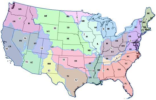 Figure 3
Major regions (HUC-2) represented by regional PCA adjustment factors overlain with U.S. state boundariesTo determine the regional PCA adjustment factors, OPP used the same methodology and rationale used to identify the national default PCA adjustment factor. The largest HUC-8-scale PCA adjustment factor within each major region was selected to represent the default PCA adjustment factor for that region. Like the national default PCA adjustment factor, the regional default PCA adjustment factors represent all agriculture, not individual crops. These values can be used as a refinement of drinking water exposure for specific regions of the country for crops other than the major crops, as defined above. Table 2 shows the maximum default PCA adjustment factors for each of the 18 major regional basins.
Table 2
Maximum percent cropped area (PCA) adjustment factor for each region
(locations in Figure 3)Location Regional Basin Regional Basin Name Default Regional PCA East of Eastern Divide 01 New England 14 02 Mid Atlantic 46 03 South Atlantic - Gulf 38 Mid-Continent (Mississippi River Basin) 04 Great Lakes 77 05 Ohio 82 06 Tennessee 38 07 Upper Mississippi 85 08 Lower Mississippi 85 09 Souris - Red - Rainy 83 10 Missouri 87 11 Arkansas - White - Red 80 12 Texas Gulf 67 13 Rio Grande 28 West of Western Divide 14 Upper Colorado 7 15 Lower Colorado 11 16 Great Basin 28 17 Pacific Northwest 63 18 California 56 -
-
Guidance for Use
National Scale Assessments
For a national-scale drinking water exposure assessment using the index reservoir scenario, surface water source estimated pesticide concentrations (peak and long-term average) will need to be adjusted (reduced) by the relevant PCA (Table 1). This is done by post-processing the modeled values.
Note that there is an entry for "All Agricultural Land" in Table 1. This is a default value to use for crops without a specific PCA adjustment factor (e.g., crops other than corn, soybeans, wheat, and cotton). This default value is also used when a pesticide is applied to multiple crops which may include but are not limited to corn, soybeans, wheat, and cotton. The PCA adjustment factor represents the largest amount of land in agricultural production in any 8-digit HUC unit in the coterminous United States. PCA adjustment factors are not applicable for non-agricultural uses (e.g., rights of way, ornamentals, turf, etc.); exposure estimates for uses that include non-agricultural uses are not reduced, as data on non-agricultural uses were not available and therefore were not used to develop PCA adjustment factors. Similarly, PCA adjustment factors are not applicable to areas outside the coterminous United States (e.g., Alaska, Hawaii, and Puerto Rico).
Selection of PCA adjustment factors depends on the degree of refinement of the exposure assessment and on the crops modeled. Regarding crops, estimates may be developed for the following situations:
-
a single crop without a PCA adjustment factor or multiple crops that are not limited to crops with PCA adjustment factors;
-
a single crop that has a crop-specific PCA adjustment factor; and
-
multiple crops that all have crop-specific PCA adjustment factors.
A decision tree for this process is provided in Figure 4. A discussion of these three situations is provided below.
-
If the pesticide is applied to a single crop without a PCA adjustment factor, multiply the peak and long-term average unadjusted estimated drinking water concentrations (EDWC) for the crop by the national default PCA adjustment factor to obtain the final EDWC. If the pesticide is applied to multiple crops which are not limited to only corn, soybeans, wheat, and cotton, multiply the peak and long-term of the highest average unadjusted EDWC by the national default PCA adjustment factor to obtain the final EDWC. If the pesticide is used for non-agricultural purposes (e.g., rights of way, ornamentals, turf, etc.), the national default PCA adjustment factor is 1.0; otherwise, the national default PCA adjustment factor is 0.87.
-
If the pesticide is only registered for use on a single crop with a developed PCA adjustment factor (corn, wheat, soybeans, or cotton), multiply the peak and long-term average unadjusted EDWCs by the appropriate PCA adjustment factor for that crop (Table 1) to obtain the final EDWCs. For Tier 2 modeling, the PCA adjustment factor should be applied regardless of where the modeled scenario is located, since the PCA adjustment factor represents the maximum national percent cropped area for that particular crop. As an example, for a pesticide used only on corn, the PRZM/EXAMS EDWCs should be multiplied by 0.46, regardless of the location of the PRZM/EXAMS corn scenario used in modeling.
-
If the pesticide is registered only for use on multiple crops for which crop-specific PCA adjustment factors have been developed (corn, wheat, soybeans, or cotton), multiply all of the peak and long-term average unadjusted EDWCs by the PCA adjustment factor for the crop combination (Table 1) to obtain the final EDWCs. The PCA adjustment factor that should be used represents the maximum potential percentage of the watershed that could be planted with these crops. If, for example, a pesticide is only used on corn, then the assumption that no more than 46% of the watershed (at the current HUC scale used) would be planted with corn is likely to hold true. However, if the pesticide is used on both corn and soybeans, then this assumption no longer holds true, since watersheds often contain both crops with a PCA adjustment factor representing up to 83% (Table 1). In this case, the model estimates for this use should be re-adjusted to reflect the combined PCA of 0.83.
As a refinement, PCA adjustments can be applied to the full time series generated by PRZM/EXAMS in a Tier 2 assessment in order to further refine the dietary assessment. The Water Quality Technology Team (WQTT) Advisory "Guidance on Generating Drinking Water Distribution Files for HED's Dietary Risk Assessments" provides instructions for preparing PCA-adjusted EDWC distributions for input into probabilistic dietary models (see Appendix A).
Regional Refinements
If dietary risks are exceeded in the national scale assessment, the risk manager may ask EFED to refine the pesticide exposure assessment. The risk assessor can either refine the assessment qualitatively by providing additional characterization of potential exposure, or quantitatively by simulating additional sites for each crop, or by using regional PCA adjustment factors in the estimation of the EDWCs. The most appropriate use of regional PCA adjustment factors can be best determined in discussions between risk assessors and risk managers. Possible options that can be considered include the following:
-
Use regional default PCA adjustment factors to refine EDWCs for uses with limited regional extent, such as Section 18 emergency exemptions, Section 24(c) Special Local Need requests, or crops with limited, well-defined growing regions (e.g., citrus).
-
Use regional PCA adjustment factors to better distinguish which crop-chemical scenarios in a pesticide use area may result in the highest surface-water EDWCs. For instance, a crop with a small percentage of total usage of the pesticide grown in the South Atlantic-Gulf basin may have a maximum use rate much higher than the predominant usage on corn in the Midwest. However, after application of the regional PCA adjustment factor to the minor use scenario, the EDWC from the Midwest corn scenario might be higher and, therefore, the driver of the drinking water exposure assessment.
-
Use regional PCA adjustment factors in association with a pesticide usage map to distinguish between the magnitudes of possible exposures for the same crop in different regions of the country and to focus spatial modeling refinements. For instance, EDWCs from a Maine potato scenario may be greater than those from an Idaho potato scenario if the same national PCA adjustment factor was applied to both. However, applying the regional default PCA adjustment factors (14% for Maine and 63% for Idaho) may lead the risk assessor and risk manager to focus on the use in Idaho. This in turn may help risk managers focus mitigation actions on regions where the greatest exposure is likely to occur.
-
Use regional PCA adjustment factors to populate a matrix of regional peak or chronic EDWCs for each labeled use of a pesticide that is expected to result in dietary risk exceedances in order to refine a drinking water exposure assessment. Begin by tabulating states by HUC-2 region where labeled crops are grown and geographically allowed for use. Then, assign PRZM/EXAMS scenarios or surrogates for each HUC-2 region for which exposure will be estimated. Next, model the maximum labeled use pattern (which may be geographically specific) for each use and tabulate the regional PCA-adjusted point EDWCs. The risk assessor may request from HED a back-calculated drinking water level of concern (DWLOC) for reference (e.g., highlight on the table EDWCs that exceed the DWLOC).
As an additional refinement, for uses with regional PCA-adjusted EDWCs greater than the DWLOC, the risk assessor may request from the Biological and Economic Analysis Division (BEAD) reported use information from areas of the United States with similar geography and/or crop management practices. This information can be used to model and characterize "reported" use patterns, based on the average number of applications and high-ends of the application rate distributions reported. Characterization of these "reported" use patterns may help risk managers to determine whether use pattern reductions to levels that appear to remain efficacious, may be worthwhile label mitigations.
Although national PCA adjustment factors based on 8-digit HUCs have been peer-reviewed by the SAP, it is imperative that the risk assessor characterize the assumptions and implications when employing regional default PCA adjustment factors. While specific uncertainties, such as scale and location of cropped areas within a watershed, are common to those connected with use of the national default PCA adjustment factor, some uncertainties are magnified by a regional assessment. For instance, in regional assessments, basins along the border with Mexico (e.g., Rio Grande basin) and with Canada (e.g., Great Lakes basin) do not include those portions of the watershed outside of the United States. Depending on the intensity of agriculture across the border, the regional PCA adjustment factors may underestimate or overestimate the fraction of land in the watershed that is cropped, affecting EDWCs.
-
-
Reporting Results
Results from simulations using the index reservoir should be included in drinking water exposure assessments. The assessments should highlight the set of values representing a single or multiple crops used in dietary risk assessments, generally those that resulted in the highest EDWCs. An example table, which can be used to summarize the EDWCs used for drinking water exposure, is presented below (Table 3). In the body of drinking water memoranda, describe the approach used, report the values for each crop simulated, and the PCA adjustment factors used (include these values in an input table).
Table 3
Example table for reporting EDWCs in drinking water exposure assessmentsTable X. Estimated drinking water concentrations (EDWCs) resulting from major use pattern applications of Chemical X. Drinking water source
(model)Use
(modeled rate)1-in-10 year peak
(µg/L)1-in-10 year annual mean
(µg/L)Overall mean
(µg/L)Surface water (PRZM/EXAMS) Use 1 Use 2 Use 3 Use 4 Groundwater (SCI-GROW) Use 1 Use 2 Use 3 Use 4 The following explanation should be included with the EDWC estimates:
Drinking water modeling involves field-scale simulations that treat watersheds as large fields. The scenarios assume that the entire area of the watershed is planted with the crop of interest (i.e., 100% crop coverage). This assumption may not hold for areas larger than a few hectares, such as watersheds containing drinking water reservoirs. Therefore, estimated drinking water concentrations were adjusted by a factor that represents the maximum percent cropped area found for the crop or crops being evaluated.
Percent cropped area (PCA) adjustment factors were derived on a watershed basis with GIS tools using the 1997 Census of Agriculture data and 8-digit Hydrologic Unit Code (HUC) coverage for the conterminous United States. The maximum PCA derived from this project was selected to represent the modeled crop or crops. The PCA assumes the distribution of each crop within a county is uniform and homogeneous. Distance between the treated fields and the water body is not addressed.
Below is standard language for describing the uncertainties in using modeling with the index reservoir and PCA adjustment factor for describing the exposure to pesticides in surface water source drinking water.
-
The PCA is a watershed-based modification. Implicit in its application is the assumption that currently used field-scale models reflect basin-scale processes consistently for all pesticides and uses. In other words, it is assumed that the large field simulated by the index reservoir models is a reasonable approximation of pesticide fate and transport within a watershed that contains a drinking water reservoir. If the models fail to capture pertinent basin-scale fate and transport processes consistently for all pesticides and all uses, the application of a factor that reduces the concentrations estimated by modeling could, in some instances, result in underestimated EDWCs. Important basin scale processes that are not simulated by using PRZM and EXAMS with a PCA factor tend to reduce the peak concentration below the estimate, but may extend the duration of its occurrence. Examples of these processes include applications to different fields on different dates, non-simultaneous entry of runoff into the water body at different locations in the watershed, and subsurface interflow through ground water.
-
The spatial data used for the PCA came from readily available sources and have a number of inherent limitations:
-
The size of the 8-digit HUC [mean = 366,989 ha; range = 6.7-2,282,081 ha; n = 2,111] may not provide reasonable estimates of actual PCAs for smaller watersheds. The watersheds that drain into drinking water reservoirs are generally smaller than the 8-digit HUC and may be better represented by watersheds defined for drinking water intakes.
-
The conversion of the county-level data to watershed-based percent cropped areas assumes the distribution of the crops within a county is uniform and homogeneous throughout the county area. Distances between the treated fields and the water body are not addressed.
-
PCA adjustment factors were generated using data from the 1992 and 1997 Census of Agriculture. The assumption that "yearly changes in cropping patterns will cause minimal impact" remains a source of uncertainty.
-
The PCA adjustment factors do not consider the percent of the crop treated in the watershed because detailed pesticide usage data are extremely limited at this time and are currently available for only a few states.
-
-
-
Literature Cited
Effland, William R., Thurman, Nelson C., and Kennedy, Ian. 1999. Proposed Methods For Determining Watershed-Derived Percent Crop Areas And Considerations For Applying Crop Area Adjustments To Surface Water Screening Models. Presentation to the FIFRA Science Advisory Panel, May 27, 1999.
Jones, R. David and Abel, Sidney. 1997. Use of a Crop Area Factor in Estimating Surface-Water-Source Drinking Water Exposure. Presentation to the FIFRA Science Advisory Panel, December, 1997.
OPP. 2002. Organophosphate Pesticides: Revised Cumulative Risk Assessment. Revised assessment released June 10, 2002.
SAP. 1999. Report: FIFRA Scientific Advisory Panel Meeting, May 25-27, 1999, held at the Sheraton Crystal City Hotel, Arlington, Virginia. Sets of Scientific Issues Being Considered by the Environmental Protection Agency Regarding: Session III - Use of Watershed-derived Percent Crop Areas as a Refinement Tool in FQPA Drinking Water Exposure Assessments for Tolerance Reassessment. SAP Report No. 99-03.
Seaber, Paul R., Kapinos, F. Paul, and Knapp, George L. 1987. Hydrologic Unit Maps. United States Geological Survey Water-Supply Paper 2294. United States Geological Survey, Denver, Colorado.
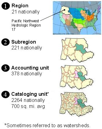
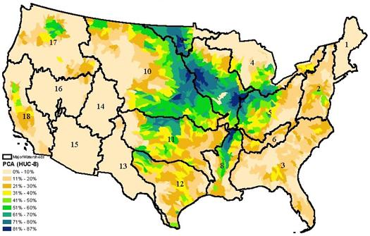

 Figure 4
Decision tree for national PCA adjustment factor determination
Appendix A
WQTT Advisory Memorandum
| DATE: | May 9, 2007 |
|---|---|
| SUBJECT: | WQTT Advisory Note: Guidance on Generating Drinking Water Distribution Files for HED's Dietary Risk Assessments |
| FROM: | Nelson Thurman, Senior Scientist Environmental Fate and Effects Division (7507C) Office of Pesticide Programs |
| TO: | Water Quality Technical Team Environmental Fate and Effects Division (7507C) Office of Pesticide Programs |
| THRU: | Dirk F. Young, Ph.D., WQTT Chair Greg Orrick, WQTT Chair Betsy Behl, WQTT Management Representative |
While preliminary drinking water assessment tiers currently compare a single one-in-ten year peak concentration to a drinking water level of comparison (DWLOC) value, current dietary exposure models used by HED (DEEM/CALENDEX, CARES, Lifeline) can accommodate distributions of drinking water concentrations (chemographs). For acute endpoints, HED is requesting that EFED provide full distributions of estimated drinking water concentrations with time. In order for HED to import the distribution into their models, the data must be in a certain format: comma delimited date and water concentration in parts per million (ppm). This document provides guidance on how to convert PRZM/EXAMS time series outputs into the appropriate format. The steps assume the use of the EFED PE shell.
Required Format for Drinking Water Distribution Files
-
Comma-delimited (.csv)
-
NO HEADER
-
1st column: Date in MM/DD/YYYY
-
2nd column: concentration in ppm
-
NO ADDITIONAL COLUMNS
Steps to Convert Time Series File to Required Format
NOTE: These steps are required because the current PE4 shell does not automatically generate the time series in the required format; nor does it adjust drinking water concentrations by percent crop area (PCA). Hopefully, future versions of the shell will do this automatically, rendering this guidance unnecessary. But we're not there yet.
-
Run PRZM/EXAMS for the drinking water assessment using the Index Reservoir. With the PE4 shell, a time-series file is generated. Look for the file that ends with *_TS.out. This is the time-series file. With the current met files, this file will be in the neighborhood of 350-400kb in size. NOTE: If you've already run PRZM/EXAMS for the 1-in-10-year concentrations, the time series file already exists.
-
Open the file in Excel. You can import it if you wish or you can start with Excel open and, using Explorer, drag the TS file and drop it into Excel.
-
You'll end up with a dataset that looks something like the table below with 4 columns:
- day numbered consecutively,
- date in MM/DD/YYYY,
- concentration in water (ppm) in scientific notation, and
- benthic sediment concentration (ppm). Unless you specified that benthic concentrations be generated, that column will probably be populated with zeros.
day date conc (ppm benthic co 0 1/1/1961 0.00E+00 0.00E+00 1 1/2/1961 0.00E+00 0.00E+00 2 1/3/1961 0.00E+00 0.00E+00 3 1/4/1961 0.00E+00 0.00E+00 4 1/5/1961 0.00E+00 0.00E+00 5 1/6/1961 0.00E+00 0.00E+00 6 1/7/1961 0.00E+00 0.00E+00 ... 10952 12/27/1990 2.19E-04 0.00E+00 10953 12/28/1990 2.17E-04 0.00E+00 10954 12/29/1990 2.14E-04 0.00E+00 10955 12/30/1990 2.12E-04 0.00E+00 10956 12/31/1990 2.10E-04 0.00E+00 -
You only need the date and water concentration concentrations, so delete the 1st (day) and 4th (benthic conc) columns. Also delete the first, header, row. HED's programs will be looking for values in the 1st line. The resulting data should look like the table below.
day conc(ppm) 1/1/1961 0.00E+00 1/2/1961 0.00E+00 1/3/1961 0.00E+00 1/4/1961 0.00E+00 1/5/1961 0.00E+00 1/6/1961 0.00E+00 1/7/1961 0.00E+00 12/27/1990 2.19E-04 12/28/1990 2.17E-04 12/29/1990 2.14E-04 12/30/1990 2.12E-04 12/31/1990 2.10E-04 -
Multiply the water concentration number by the PCA (percent crop area, expressed as a decimal fraction). This can be done in several ways; these instructions illustrate one quick and easy way of doing this:
-
In an adjacent cell, enter the pca as a decimal fraction (for instance, the default pca would be 0.87). Select the cell and copy the value.
-
Highlight the drinking water concentration column (select the entire distribution/column).
-
Right-click on the highlighted column, select "Paste special", and select the "Multiply" option. Select OK. This converts the entire distribution to the pca-adjusted value.
-
You might need to format the concentration column into scientific notation (2 decimal places). The resulting distribution, shown below, reflects a default pca-adjustment of 0.87.
day conc(ppm) 1/1/1961 0.00E+00 1/2/1961 0.00E+00 1/3/1961 0.00E+00 1/4/1961 0.00E+00 1/5/1961 0.00E+00 1/6/1961 0.00E+00 1/7/1961 0.00E+00 12/27/1990 1.91E-04 12/28/1990 1.89E-04 12/29/1990 1.86E-04 12/30/1990 1.84E-04 12/31/1990 1.83E-04 -
-
Once you've done that, save the distribution as a comma-delimited file by
-
clicking on "Save as..." in the File menu,
-
selecting "CSV (comma delimited)(*.csv)" as the "Save as type", and
-
giving it an appropriately descriptive name so you know what it is and could track it down again. If you pull it up in a text editor, it'll look like this:
day,conc(ppm) 1/1/1961,0.00E+00 1/2/1961,0.00E+00 1/3/1961,0.00E+00 1/4/1961,0.00E+00 1/5/1961,0.00E+00 1/6/1961,0.00E+00 1/7/1961,0.00E+00 ... 12/27/1990,1.91E-04 12/28/1990,1.89E-04 12/29/1990,1.86E-04 12/30/1990,1.84E-04 12/31/1990,1.83E-04 -
-
That's all there is to it. This file, in this format, will be pulled into HED's dietary exposure models.