N-STEPS - Nutrient and Response Variable Overviews
You may need a PDF reader to view some of the files on this page. Refer to EPA’s About PDF page to learn more.
Descriptions of common nutrient (e.g., nitrogen) and response variables (e.g., phytoplankton) and sampling methods for these variables. Select a variable for more information. Additional resources for variables and sampling methods are included.
Clarity
Clarity is a measure of the amount of sunlight that can penetrate through the water column, reflecting the amount of dissolved colored or suspended material in any waterbody. Clarity can be affected by natural and introduced materials. Clarity can be the result of, as well as a limitation to, productivity. Suspended algae contribute to reduced water clarity, which at the same time can limit light available to growth of algae at depth. In streams and lakes, inorganic sediment can also contribute to reduced clarity. Although usually the case following storms, some waters do maintain high inorganic sediment loads even during baseflow. In the context of nutrient criteria, the utility of clarity measures is related to contributions from suspended algal material in the water column. This material can come from true phytoplankton or from tychoplankton (algae dislodged or sloughed from the benthos). In either case, significant correlations have been drawn between the amount of algae in the water column and its clarity, especially for lakes. One of the common trophic indices for lakes, the Trophic State Index (TSI), can be derived using a measure of transparency. Clarity may have limitations as a nutrient endpoint as reduced clarity is often caused by non-nutrient issues such as waste discharges, runoff from watersheds, soil erosion, and humic acids and other organic compounds resulting from the decay of plants and leaf litter.
Clarity can be measured in a number of ways. One of the traditional lake quality measures is the vertical Secchi depth transparency measurement, which was adapted from a method developed by an Italian papal advisor, Father Pietro Angelo Secchi, in the 19th century. Similar horizontal adaptations of transparency measures have been tested for streams and rivers. A similar measure to clarity is turbidity, which measures the scatter and absorption of light by suspended particles. Another way to evaluate turbidity is to directly measure the total suspended material gravimetrically. These measures are fairly convenient and, with the exception of gravimetric suspended solids, can be directly measured in the field.
For estuaries, water clarity has been a concern implicated in the decline of seagrass diversity, density, and distribution. The best measure of light attenuation, of particular importance to seagrasses, is direct measure of photosynthetically active radiation (PAR) to generate a light attenuation coefficient (Kd). Relationships have been developed to help convert between Secchi depths and Kd for specific estuaries.
Transparency
Transparency is traditionally measured using light meters and is quantified with light extinction coefficients. However, this is rarely done in routine water quality monitoring. For lakes, the most common method is deploying a Secchi disk. There is not a common method used for streams and rivers, although a horizontal transparency method has been tested.
Secchi Transparency
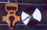
The Secchi disk is a weighted white or black and white disk, 20 cm in diameter that is attached to a graduated line. The disk is lowered over the shaded side of a boat, ideally at midday, and the average of the depths at which the disk disappears and reappears is the estimate of Secchi transparency. Transparency is a function of the reflectance of light from the disk. Any dissolved color or suspended materials that absorb or scatter light will reduce the Secchi transparency, so Secchi depth is proportional to transparency. Transparency measured with Secchi disks is correlated with transmissivity measured directly with photometers, and the Secchi depth is usually around the 10 to 15 percent transmission point. Secchi depth in lakes, especially in the absence of color or inorganic suspended material, is highly correlated with algal biomass and can be used to calculate the TSI, which is an accurate measure of lake trophic status. Secchi depths range from a few centimeters in very turbid lakes to over 40 m in clear, oligotrophic lakes, but most are in the range of 2 to 10 m. There is no comparable routine transparency measure used in streams; however, horizontal black disk samplers have been developed.
Turbidity
Turbidity is a measure of the scatter of light by particles in suspension. It is not the same as clarity and is, in fact, an inverse measure of clarity. Turbidity is caused by suspended particles that intercept light and refract, reflect, or diffract it. These particles include algal cells and high concentrations of water column algae, whether true plankton or dislodged benthic algae (tychoplankton), which will increase turbidity. The Jackson candle turbidimeter was the historical method of choice (units – the Jackson Turbidity Unit or JTU); however, nephelometers have replaced those due to their greater sensitivity.
It is important to note that, historically, turbidity units [both Nephelometric Turbidity Units (NTUs) and Formazin Nephelometric Units (FNUs)] were considered one and the same, but current practices separate the units based on method. Measurements complying with USEPA Method 180.1 are reported in NTUs, whereas those complying with ISO 7027 are reported in FNUs. Current practices retain the use of NTUs and FNUs, but their use is restricted to data from instruments that conform to the specific designs defined in USEPA Method 180.1 and ISO 7027, respectively.
Nephelometry
Nephelometers are turbidimeters that measure light scatter at 90 degrees to the incident light beam. Both bench-top and portable nephelometers are available and can give fairly precise and accurate measures, if calibrated properly and regularly. A nephelometer compares the intensity of light scattered by a sample relative to a standard. The greater the scatter, the higher the turbidity, measured as NTUs. Formazin polymer is commonly used in standard reference suspensions. Continuous nephelometers, which can be deployed in the field for long periods of continuous turbidity measurement, are available. Turbidities in the range of 0 to 40 NTU can be measured directly with a nephelometer. Higher values should be diluted to this range, measured, and final concentrations estimated appropriately.
Continuous Monitoring
Turbidity measurements under dynamic water conditions are most commonly taken by submersible sensors, using either instantaneous profiling techniques or a deployed instrument for continuous monitoring. Turbidity sensors for most submersible continuous water-quality sondes are based on nephelometric near-infrared wavelength technology that is compliant with ISO 7027. Data should be reported in FNUs. Routine maintenance of turbidity instrumentation is critical, especially for continuously deployed, dynamic applications. Instrument drift and fouling are two main issues.
Literature Cited
Anderson, C.W. 2004. Turbidity (version 2.0): U.S. Geological Survey Techniques of Water-Resources Investigations, book 9, chap. A6, section 6.7, 64 p.
APHA. 1999. Standard Methods for the Examination of Water and Wastewater. 20th edition. American Public Health Association, Washington, DC.
Carlson, R.E. 1977. A trophic state index for lakes. Limnology and Oceanography 22:361-369.
Davies-Colley, R.J. and D.G. Smith. 2001. Turbidity, suspended sediment, and water clarity: A review. Journal of the American Water Resources Association 37:1085-1101.
Dennison, W.C., R.J. Orth, K.A. Moore, J.C. Stevenson, V. Carter, S. Kollar, P.W. Bergstrom, and R.A. Batiuk. 1993. Assessing water quality with submersed aquatic vegetation. BioScience 43 (2):86-94.
Duarte, C.M. 1995. Submerged Aquatic Vegetation in Relation to Different Nutrient Regimes. Ophelia 41:87-112.
Lee, K., S.R. Park, and Y.K. Kim. 2007. Effects of irradiance, temperature, and nutrients on growth dynamics of seagrasses: A review. Journal of Experimental Marine Biology and Ecology 350 (1-2):144-175.
USEPA. 2012. Water Monitoring and Assessment. 5.5 Turbidity. U.S. Environmental Protection Agency
USGS. 2004. Office of Water Quality Technical Memorandum 2004.03, Revision of NFM Chapter 6, Section 6.7—Turbidity. U. S. Geological Survey.
Wagner, R.J., R.W. Boulger Jr., C.J. Oblinger, and B.A. Smith. 2006. Guidelines and Standard Procedures for Continuous Water-quality Monitors—Station Operation, Record Computation, and Data Reporting: U.S. Geological Survey Techniques and Methods. 1–D3, 51 p. + 8 attachments.
Wetzel, R.G. and G.E. Likens. 2000. Limnological Analyses. 3rd edition. Springer-Verlag, New York.
Dissolved Oxygen
Dissolved oxygen (DO) is a measure of how much oxygen is dissolved in water and potentially available to aquatic organisms for respiration (commonly measured in mg/L). The saturation level of oxygen in freshwater at 20°C and 1 atm of atmospheric pressure is 9.1 mg/L, and DO decreases with increased water temperature, altitude, and salinity. Annual cycles in DO concentration are normally observed due to seasonal temperature changes. One way that oxygen enters or leaves the water column is through diffusion across the surface, with subsequent advection (circulation) of oxygen-rich surface waters to deeper areas. Physical features such as rapids, waterfalls, and riffles increase surface area, aeration, and DO levels. Oxygen also enters water during photosynthesis by phototrophs. Oxygen is consumed by aquatic organisms, decomposition of organic material, and multiple chemical reactions.
Although DO requirements vary among species, life stages, and a number of other factors, sufficient DO is essential for growth and reproduction of aerobic aquatic life. Hypoxic waters, characterized as waters having a DO concentration less than 2 mg/L, generally result in adverse chronic or acute effects including reduced reproduction, lower growth, altered foraging patterns, spatial avoidance, migration of fish and mobile benthic invertebrates, and death. Hypoxia and anoxia in bottom waters can also result in anoxia in surface sediment, sometimes creating reducing zones that result in the release of toxic hydrogen sulfide (H2S), soluble reactive phosphorus (SRP), and ammonia (NH3). As a result, anoxic sediment can be a source of nutrients.
Diurnal Cycle
Algae and macrophytes increase DO concentrations in the photic zone as a result of photosynthesis during the day, but they decrease DO concentrations at night when respiration continues in the absence of photosynthesis. As a result, DO fluctuates over a 24-hour cycle, increasing during daylight hours when photosynthesis is occurring and reaching minimum values just before dawn. The diurnal variations can be significant in eutrophic systems with DO levels exceeding saturation during the day but reaching levels low enough to cause harm to aquatic life, including massive die-offs of aquatic animals such as fish overnight. The epilimnion (surface layer during stratification) of eutrophic lakes shows greater swings in DO concentrations than in less productive lakes, due to the diurnal shift between algal photosynthesis and respiration. Conditions (e.g., during a severe algae bloom) may favor development of extremely low DO levels overnight.
Stratification
Low dissolved oxygen levels are common in aquatic systems, especially in the bottom waters of stratified lakes, estuaries, and coastal marine systems that have high nutrient inputs. Thermal stratification in lakes occurs after surface waters are rapidly heated, and mixing (primarily from wind) is not sufficient to maintain complete circulation of the water column. As the surface waters are heated, they become less dense than cooler waters underneath, and the thermal resistance to mixing prevents complete circulation. Eutrophication affects water quality in stratified lakes, specifically dissolved oxygen dynamics and nutrient cycling.
In estuaries, salinity gradients are a common cause of stratification (e.g., Diaz 2001), where lighter, fresh water flows in on top of denser and more saline water. As with lakes, temperature can also be a contributing factor to estuarine stratification (e.g., Stanley and Nixon 1992), where warm, lighter surface water (heated by sunlight) overlies denser, cooler water. DO can fluctuate widely over a period of several hours, due to wind-induced mixing, tides, wind-induced seiches, and diurnal cycles. Tides and seiches can move low-DO bottom water into nearshore zones (e.g., Breitburg 1990); daytime photosynthesis increases DO and nighttime respiration decreases DO (e.g., Breitburg 1990), and the onset of wind can mix an unstratified but stagnant body of water, increasing reaeration.
Measuring Dissolved Oxygen
There are two principal methods for measuring DO: (1) a DO meter and (2) the iodometric (or Winkler) method. A DO meter is an electronic device that converts signals from a probe that is placed in the water into units of DO in milligrams per liter. The probe is filled with a salt solution and has a selectively permeable membrane that allows DO to pass from water into the salt solution. The DO that has diffused into the salt solution changes the electric potential of the salt solution and this change is sent by electric cable to the meter, which converts the signal to milligrams per liter on a readable scale.
DO meters are often used to continuously measure DO levels as part of real-time water quality monitoring programs. Real-time monitoring captures short-term and long-term changes in water quality including diurnal and seasonal trends in DO concentrations. Membrane sensors are deployed in the field and data are logged onsite. When configured with telemetry, data can be transmitted in real-time from a remote site to a project computer or website. DO meters, whether used for single measurements or used to continuously monitor DO, are often paired with temperature, pH, and conductivity measurements. Fouling is a concern for deployed probes.
The iodometric (or Winkler) method is a titrimetric procedure based on the oxidizing property of DO. The iodometric test fixes the DO using reagents to form an acid compound that is titrated. Titration involves the incremental addition of a reagent that neutralizes the acid compound and causes a change in the color of the solution (through use of a starch indicator). The point at which the color changes is the "endpoint" and is equivalent to the amount of oxygen dissolved in the sample.
Literature Cited
APHA. 1999. Standard Methods for the Examination of Water and Wastewater. 20th edition. American Public Health Association, Washington, DC.
Breitburg, D.L. 1990. Near-shore hypoxia in the Chesapeake Bay: Patterns and relationships among physical factors. Estuarine, Coastal and Shelf Science, 30(6):593-609.
Breitburg, D.L., T. Loher, C.A. Pacey, and A. Gerstein. 1997. Varying effects of low dissolved oxygen on trophic interactions in an estuarine food web. Ecological Monographs 67(4):489-507.
Diaz, R.J. 2001. Overview of hypoxia around the world. Journal of Environmental Quality 30(2):275-281.
Diaz, R.J. and R. Rosenberg. 2008. Spreading dead zones and consequences for marine ecosystems. Science 321(5891):926-929.
Domenici, P., C. Lefrancois, and A. Shingles. 2007. Hypoxia and the antipredator behaviours of fishes. Philosophical Transactions of the Royal Society 362:2105-21.
Howell, P. and D. Simpson. 1994. Abundance of marine resources in relation to dissolved oxygen in Long Island Sound. Estuaries 17(2):394-402.
Jones, J.R., M.F. Knowlton, D.V. Obrecht and J.L. Graham. 2011. Temperature and oxygen in Missouri reservoirs. Lake and Reservoir Management, 27(2):173-182.
McCarthy, M., K. McNeal, J. Morse, and W. Gardner. 2008. Bottom-water hypoxia effects on sediment–water interface nitrogen transformations in a seasonally hypoxic, shallow bay (Corpus Christi Bay, TX, USA). Estuaries and Coasts 31(3):521-531.
Nürnberg, G.K. 1995. Quantifying anoxia in lakes. Limnology and Oceanography 406(6):1100-1111.
Stanley, D.W., and S.W. Nixon. 1992. Stratification and bottom-water hypoxia in the Pamlico River Estuary. Estuaries 15(3):270-281.
Wagner, R.J., R.W. Boulger Jr., C.J. Oblinger, and B.A. Smith. 2006. Guidelines and Standard Procedures for Continuous Water-quality Monitors—Station Operation, Record Computation, and Data Reporting: U.S. Geological Survey Techniques and Methods. 1–D3, 51 p. + 8 attachments.
Wannamaker, C.M. and J.A. Rice. 2000. Effects of hypoxia on movements and behavior of selected estuarine organisms from the southeastern United States. Journal of Experimental Marine Biology and Ecology 249:145–163.
Wetzel, R.G. 2001. Limnology: Lake and River Ecosystems. 3rd edition. Academic Press, New York.
Nitrogen
Nitrogen can be a limiting nutrient in both marine and freshwater environments (e.g., Elser et al. 2007), despite previous ideas about it primarily limiting marine systems (e.g., Howarth, 1988). Excess nitrogen in surface waters can lead to eutrophic conditions, which can impact the health of aquatic systems. In addition, some forms of nitrogen can be harmful to human health. A common example is nitrate in drinking water. Anthropogenic sources of nitrogen to aquatic systems include fertilizers (from suburban and agricultural runoff), animal and human waste, and atmospheric deposition.
Nitrogen exists in a number of different valence states, one reason for the variety of biogeochemical reactions that occur as part of the nitrogen cycle. Typical measures of nitrogen include total nitrogen, total organic nitrogen, nitrate, nitrite, and ammonia. The inorganic forms nitrate and ammonia are most readily available for uptake in aquatic systems.
Total nitrogen refers to the total amount of nitrogen in a water sample, which typically contains a variety of inorganic and organic forms. Total nitrogen can be determined by complete oxidation of all forms with a strong oxidant (such as persulfate) and then determination of the nitrate concentration.
Organic nitrogen (including amino acids, peptides, proteins, nucleic acids, and urea) is defined functionally as bound nitrogen in the tri-negative oxidative state but does not include all organic forms of nitrogen. Kjeldahl nitrogen is a technique that determines organic nitrogen and ammonia (NH3) together. Organic nitrogen can be estimated by subtracting ammonia from total Kjeldahl nitrogen or by subtracting ammonia, nitrate, and nitrite from a measure of total nitrogen. Organic nitrogen occurs in the range of tens of µg N/L to more than 20 mg N/L in raw sewage.
Total oxidized nitrogen is the sum of nitrate and nitrite. Nitrate (NO3-) is the most oxidized form of nitrogen and is usually found in low concentrations in oligotrophic waters (10-100 µg -N/L) but can be in the 10 to 100 mg N/L range in biologically treated effluent or eutrophic waters. Nitrate is taken up by plants and algae and enzymatically reduced to the organic amino form with nitrate reductase. Nitrate can also be reduced by denitrification, a microbially-mediated process occurring under anaerobic conditions that uses nitrate as a terminal electron acceptor and results in the production, ultimately, of nitrogen gas (N2). Nitrite (NO2-) is an intermediate oxidative state that is usually found in low concentrations in water. However, it is used in some industrial applications, the effluent of which can contain high concentrations.
Ammonia (NH3) is the most reduced form of nitrogen. It originates naturally from the decomposition of organic nitrogen compounds and hydrolysis of urea. It is usually present in low concentrations of tens of µg N/L, except where enrichment from various sources results in concentrations in the hundreds of µg NH3-N/L to tens of mg NH3-N/L range. Concentrations of nitrogen ions are usually reported as elemental nitrogen in its various forms and NO3-N, NO2-N, and NH3-N are technically “N as nitrate, N as nitrite, and N as ammonia”. It is important to check that concentrations are given in terms of the elemental nitrogen concentration.
The following are brief descriptions of some standard methods for measuring different forms of nitrogen. Users interested in further specific and detailed methods should refer to the literature cited.
Total Nitrogen
Total nitrogen methods employ strong oxidants to convert all forms of nitrogen (reduced and oxidized, bound and dissolved) into nitrate ions. It differs from total Kjeldahl nitrogen, which does not measure oxidized forms of nitrogen.
Persulfate Digestion
The persulfate method, as mentioned above, uses the strong oxidant, persulfate, to convert all forms of nitrogen in a sample into the nitrate molecule, which most efficiently occurs at 100 to 110oC in an alkaline environment. This is usually done with digestion tubes using autoclaves, hotplates, etc. The resulting nitrate is then measured using nitrate methods after cooling and buffering the sample.
Organic Nitrogen
Organic nitrogen methods measure principally nitrogen in the tri-negative state (amino). They do not measure other organic forms of nitrogen (e.g., -azide, -azine, -azo, nitro, etc.). Organic nitrogen concentration can be elevated in areas with large potential sources of organic nitrogen without treatment and in areas with high levels of nitrogen inputs in general. Even in oligotrophic areas, organic forms may dominate the nitrogen pool. The traditional method for measuring organic nitrogen is the Kjeldahl method.
Kjeldahl Method
This method measures organic nitrogen and ammonia. The principle of this method is that amino-nitrogen compounds are converted to ammonium in the presence of sulfuric acid, potassium sulfate, and cupric sulfate during a digestion. Free ammonia (NH3) is also converted into ammonium (NH4+). After the initial digestion, base is added and the sample distilled to remove the ammonium. Ammonium is then measured using an appropriate ammonium method (e.g., phenate method). As this method commonly measures dissolved ammonia as well as organic nitrogen, organic nitrogen alone can be measured by removing the ammonia first and using a pre-distillation or subtracting the ammonia measured using a dissolved ammonia method. This method is applicable over a wide range of organic nitrogen plus ammonia concentrations but requires large volumes for low concentration waters. The macro-Kjeldahl method typically uses 800 ml Kjeldahl flasks. A micro-Kjeldahl method exists that is applicable over the range of organic plus ammonia nitrogen of 0.2 to 2 mg N/L (APHA 1999; 4500-NorgC). This method simply uses smaller volume (100 ml) Kjeldahl flasks.
Ammonia Nitrogen
Ammonia is the most reduced form of nitrogen. It usually exists in low concentrations and most often exists as the ammonium ion (NH4+) except under high pH (>9.0). Ammonia can generally be measured directly in surface water samples, although filtration can be used as well as distillation for samples with common interference or very high concentrations (> 5 mg NH3-N/L).
Phenate Method
The principal of the phenate method is that ammonium, in the presence of hypochlorite and phenol, forms an intense blue compound, indophenol, which can be measured spectrophotometrically. The amount of indophenol produced is proportional to the ammonium concentration. It is a fairly straightforward method, which is accurate to very low concentrations (0.01 mg NH3-N/L) with long path cell lengths and is linear up to 0.6 mg NH3-N/L. Samples above this concentration may have to be diluted. There is an automated form of the phenate method (APHA 1999; Method 4500-NH3 G), which follows the same principal as the manual method, but uses continuous flow analytical machines that automate the process and can be used for analyzing samples in large batches. The automated method is applicable over the range of 0.02 to 2.0 mg NH3-N/L.
Nitrite Nitrogen
Nitrite is the trivalent form of nitrogen, which usually exists in concentrations below that of nitrate. However, nitrite concentrations can be elevated, for example, in rivers under warm, slow-moving conditions or in anaerobic lake strata as a result of high rates of denitrification (dissimilatory nitrate reduction or denitrification) or in effluent from industrial applications employing nitrite.
Colorimetric Method
The principal of this method is that nitrite forms a reddish purple azo dye under acidic conditions when combined with certain reagents. This color is produced in proportion to the concentration of nitrite and can be measured spectrophotometrically. This is the common nitrite method and is useful in the range of 10 to 1,000 mg NO2-N/L. Lower concentrations can be estimated by using a 5 cm path cell. Higher concentrations should be diluted.
Nitrate Nitrogen
Nitrate is the most oxidized common form of nitrogen in freshwaters. It is taken up by algae and plants and reduced to the amino form (assimilatory nitrate reduction) and by denitrifying bacteria and converted into nitrogen gas (dissimilatory nitrate reduction or denitrification). Nitrate concentration can be quite high where nitrogen loading exists as a result of direct nitrate input or as a result of nitrification of reduced organic forms by bacteria. Nitrate measurement is difficult because of the relatively complex method and apparatus required, common interferences, and the limited range of different methods. Nitrate can be determined by ion chromatography or capillary ion electrophoresis. The more traditional technique is the cadmium reduction method.
Cadmium Reduction Method
The principal of this method is that nitrate is reduced almost completely to nitrite in the presence of cadmium. The nitrite produced is then determined following the standard colorimetric method described for nitrite above. Note that this method measures both nitrate and nitrite in the sample. Nitrite can be subtracted by measuring a subsample directly without the reduction step. The manual method is applicable across nitrate ranges from 0.01 to 1 mg NO3-N/L. Higher concentrations can be diluted. An automated version of this method exists (APHA 1999; Method 4500- NO3-F), which follows the same principal as the manual method, but uses continuous flow analytical machines that automate the process and can be used for analyzing samples in large batches. The automated method is applicable over the range of 0.001 to 10.0 mg NO3-N /L, and higher concentrations can be diluted.
Continuous Monitoring
Continuous monitoring of nitrate in aquatic systems can be achieved using field deployable sensors. Ultraviolet nitrate sensors, often used for wastewater monitoring and coastal and oceanographic studies, are now being designed specifically for freshwater applications. Optical nitrate sensors are designed on the basis that nitrate ions absorb ultraviolet light at wavelengths around 220 nanometers. Commercially-available optical nitrate sensors convert spectral absorption measured by a photometer to a nitrate concentration, using laboratory calibrations and on board algorithms. Nitrate concentrations can be calculated in real-time without the need for chemical reagents that degrade over time and are a source of waste.
Literature Cited
APHA. 1999. Standard Methods for the Examination of Water and Wastewater. 20th edition. American Public Health Association, Washington, DC.
Elser, J.J., M.E.S. Bracken, E.E. Cleland, D.S. Gruner, W.S. Harpole, H. Hillebrand, J.T. Ngai, E.W. Seabloom, J.B. Shurin, and J.E. Smithet. 2007. Global analysis of nitrogen and phosphorus limitation of primary producers in freshwater, marine and terrestrial ecosystems. Ecology Letters 10:1135-1142.
Francoeur, S.N. 2001. Meta-analysis of lotic nutrient amendment experiments: Detecting and quantifying subtle responses. Journal of the North American Benthological Society 20:358-368.
Howarth, R.W. 1988. Nutrient limitation of net primary production in marine ecosystems. Annual Review of Ecology and Systematics 19:89-110.
Pellerin B.A., B.A. Bergamaschi, B.D. Downing, J. Saraceno, J.D. Garrett, and L.D. Olsen. 2013. Optical Techniques for the Determination of Nitrate in Environmental Waters: Guidelines for Instrument Selection, Operation, Deployment, Quality-Assurance, and Data Reporting (PDF). (48 pp, 2 MB) U.S. Geological Survey Techniques and Methods 1–D5, 37 p.
Wetzel, R.G. 2001. Limnology: Lake and River Ecosystems. 3rd edition. Academic Press, New York.
Wetzel, R.G. and G.E. Likens. 2000. Limnological Analyses. 3rd edition. Springer-Verlag, New York.
Periphyton
Periphyton is the community of organisms including plants, bacteria, fungi, protozoa, and invertebrates living attached to submerged substrates. These communities compose the biofilms in waterbodies where benthic algae reside. As a result, they are the focus of sampling for algal response to nutrients and are, therefore, important in nutrient criteria development. A variety of substrates support periphyton communities and are named accordingly: epilithon (on rocks), epiphyton (on plants), epidendron or epixylon (on wood), epipsammon (on sand), epipelon (on fine sediments), and epizoon (on aquatic animals).
Epiphytic algal assemblages inhabit the external surfaces of seagrass leaves and shoots. The algae and bacteria in those assemblages are an important component of natural ecosystems, providing energy through grazers to the food web. Algal assemblage composition has been used for biological assessment of both marine and freshwater systems and in the reconstruction of historical water quality conditions using paleo-reconstruction and algal-specific water quality optima. Because many algal species are highly sensitive to water quality conditions, epiphyte assemblage composition could serve as an indicator of nutrient impacts that occur before other plant degradation or eutrophication responses.
Two basic attributes of periphyton are most often sampled: biomass and composition. Biomass is generally measured by removing periphyton from substrates and weighing the resultant organic matter, extracting the chlorophyll to provide a relative estimate of algal abundance, or counting the number of algal cells and using a biovolume conversion to estimate biomass. Algal assemblage composition typically consists of removing periphyton, preserving it, and then identifying the taxa to the lowest possible taxonomic level. However, rapid periphyton methods have been developed for doing field based assemblage assessment. Both biomass and composition can be measured from the same field samples, which are split into a subsample for biomass and one for assemblage composition.
The following is a brief review of common methods. Users interested in further specific and detailed methods should refer to the literature cited.
Sample Collection
Periphyton samples can be collected using quantitative or semi-quantitative methods and a variety of programs have developed specific methods (e.g., Barbour et al. 1999, Moulton et al. 2002). Quantitative methods consist of sampling a known area of substrate, usually with a sampling device that can isolate an area which can be removed in situ (e.g., a petri dish/spatula on sand) or by removing substrates and removing the material from a specific area. Either specific substrates can be targeted or multi-habitat samples can be taken and composited. Known area samples are best for biomass estimates, but semi-quantitative, multi-habitat samples may gather more taxa. Passive samplers can also be deployed for some period of colonization. Glass slides, the top plate of Hester-Dendy macroinvertebrate samplers, and clay tiles are all examples of samplers that have been used as passive sampling substrates for periphyton. The advantage of these is the standardized sampling area and substrate characteristics. The major disadvantage is the fact that these artificial substrates may not accurately reflect the true periphyton assemblage.Algal Biomass
Algal biomass refers to the mass of algal material within the periphyton. It can be measured gravimetrically (weighed), using chlorophyll extractions, or by converting cell count data to mass using biovolume conversions. Gravimetric measures rely on weighing the amount of organic matter within the periphyton. As it is generally prohibitive to separate algal and non-algal material for routine analysis, the mass (usually the mass after combustion called ash-free dry mass [AFDM]) can include substantial non-algal material. Some people use AFDM to chlorophyll ratios to look at the proportion of non-algal material, but this is only an approximation. The content of chlorophyll per cell varies with a number of factors: species, nutrient conditions, light condition, and temperature. Therefore, chlorophyll is not a direct measure of biomass, though it has long been used as a relative measure of algal abundance. Cell biovolumes vary by taxa, their shapes, and a number of other factors affecting cellular composition. However, if quantitative genus or species level data are collected, then biomass can generally be estimated by applying shape specific geometric volume conversions.
Ash-free dry mass
After scraping a known area, the resulting “scrapate” is diluted to a known volume and a subsample of that volume is either weighed in pre-combusted and pre-weighed crucibles or weighed following filtration through appropriate pre-weighed and pre-combusted glass fiber filters (0.5-0.7 µm pore size). Crucibles and filters are then dried, weighed for dry mass, and then combusted to remove all organic matter (e.g., 500°C) and re-weighed to estimate ash-free dry mass. Samples for AFDM can be field filtered or brought to a lab for processing. Sample preservation for AFDM is not straightforward, but samples should be handled to limit respiratory loss of organic matter [e.g., placed on ice and frozen (-20 to -60°C) if there will be a delay in processing]. Consult the different specific methods for more on sample preservation. Values are expressed as grams AFDM per unit area.
Pigment analysis
A sub-sample of material removed from substrates and usually filtered onto glass fiber filters (0.5-0.7 µm pore size) is used for pigment analysis as an indicator of algal biomass in periphyton. The composition of photosynthetic pigments varies by algal taxa, but chlorophyll a is the principal pigment used because it is the most common and abundant. Chlorophylls b and c and the carotenoids absorb light at different wavelengths and can be quantified as well, if desired. Chlorophyll a degrades into different phaeopigments that absorb at the same wavelength as chlorophyll a. For this reason, chlorophyll concentration is usually measured in a sample after extraction, acidified to convert all the chlorophyll to phaeopigments, remeasured, and chlorophyll a concentration is determined by difference. Chlorophyll a is historically and most commonly measured using spectrophotometry, although fluorometry is more sensitive and becoming more commonly used.
Chlorophyll and other photopigments must be extracted from algae to quantify biomass using pigment analysis. It is best to work in low light to avoid degradation. While a variety of extraction solvents exist, alkaline aqueous acetone is still the standard recommended method (APHA 1999). Algae retained on glass fiber filters (0.5-0.7 µm pore size) are typically ground in aqueous acetone, allowed to sit for a period of time for extraction in the dark and under refrigeration, and the ground filter solution is centrifuged to separate the filter from the pigments. Pigments are then decanted and measured directly either with spectrophotometry or fluorometry. The flourometric method is usually standardized using spectrophotometric measurement of a chlorophyll extract. Fluorometry is more sensitive to low concentrations and should give comparable estimates. Consult an appropriate methods source for details on the use of either of these detection methods, including appropriate detectors and wavelengths.
Preservation of samples for chlorophyll is important. Filtration should occur as soon as possible and chlorophyll should be extracted from filters as soon as possible. Field filtration is ideal. Addition of magnesium carbonate either to the sample solution or on top of the filter after filtration has been advocated to reduce acidity, since acidity degrades chlorophyll. Filters that will not be analyzed immediately, should be folded in half, placed into labeled dark containers (i.e., wrapped in aluminum foil), and placed on ice or immediately frozen. Pigment samples may be frozen for a few days (at -20 to -60°C) but should be analyzed as soon as possible, since degradation of chlorophyll does occur.
Biovolume
Biovolume is determined by multiplying the number of each taxon identified in a sample by the average biovolume of that taxon, calculated using equations of geometric shapes most approximating that taxon, and summing these values across all the taxa in a sample. Equations for many different taxa have already been developed (Hillebrand et al. 1999), or general equations may be applied. This approach obviously requires more effort, since individual taxa must not only be counted but average dimensions must be calculated for each as well (average of 20 individuals is recommended; APHA 1999). This method does, however, offer one of the more accurate measures of live algal biomass.
Visual Estimate
As part of a field-based rapid periphyton survey developed for use in the Rapid Bioassessment Protocols, a quick visual estimation of algal biomass was developed. This approach uses gridded view buckets to visually estimate macroalgal biomass and microalgal cover. While not as accurate as actual measures of algal biomass, the technique does allow rapid relative estimates of composition and standing crop or biomass.
Algal Composition
The composition of the algal assemblage in stream periphyton can provide information about the physical and chemical environment. Unlike simple grab samples of water, the assemblage of algae integrate water quality conditions over long periods of time. Each taxon has specific optima for the wide variety of physical and chemical conditions to which periphyton are exposed, including sensitivities or tolerance to nutrients, acidity, temperature, oxygen, silt, and other variables. The average environmental conditions influence which taxa survive and thrive in a stream. As a result, a great deal of environmental information can be inferred from which algae are found in the periphyton, including nutrient conditions. The composition of algae is usually determined with microscopy, and most taxa can be identified to species by well-trained taxonomists. A rapid visual estimate of rough benthic algal composition has also been developed.
Microscopy
Unfiltered periphyton samples collected from the stream should be preserved. The preferred preservative is Lugol’s solution, but other optional preservatives include 2% M3 fixative, 4% buffered formalin, or 2% glutaraldehyde. The sample is typically homogenized with a tissue homogenizer and placed into a specific cell for viewing of large algal taxa (e.g., Palmer-Maloney or Sedgwick-Rafter cells). These can be enumerated a number of ways, but it can be difficult to enumerate colonial or filamentous individuals, and magnification is limited for these sample cells. Sedimentation chambers can also be used for identifying smaller cells if inverted microscopes are available. In this approach, a known subsample of the homogenized sample is placed into a sedimentation chamber, where the algae settle. The chamber is then placed on an inverted microscope, where greater magnification can be used to identify taxa. For diatom analysis, it is necessary to remove organic matter that might otherwise interfere with identification. This can be done with combustion or chemical oxidation of subsamples, followed by slide mounting with a suitable highly refractive medium to make permanent slides. Compound microscopy at 1000x under oil immersion is then used to identify diatoms to species. From these data, accurate identifications of the resident algal periphyton assemblage can be made. When combined with autecological information for the different algal taxa, a number of inferences about the integrated physical and chemical conditions of a stream or lake can be made.
Rapid visual estimates
The rapid visual approach uses gridded view buckets to characterize periphyton assemblages. Very coarse-level taxonomic information can be collected by individuals trained to recognize specific macro-algal taxa. The buckets are placed randomly along transects, and the algal assemblage are identified to specific macroalgal genera or to coarse algal groups (e.g., diatoms or blue-green algae).
Literature Cited
APHA. 1999. Standard Methods for the Examination of Water and Wastewater. 20th edition. American Public Health Association, Washington, DC.
Barbour, M.T., J. Gerritsen, B.D. Snyder, and J.B. Stribling. 1999. Rapid Bioassessment Protocols for Use in Streams and Wadeable Rivers: Periphyton, Benthic Macroinvertebrates and Fish, Second Edition. EPA 841-B99-002. U.S. Environmental Protection Agency, Office of Water, Washington, DC.
Cambridge, M.L., J.R. How, P.S. Lavery, and M.A. Vanderklift. 2007. Retrospective analysis of epiphyte assemblages in relation to seagrass loss in a eutrophic coastal embayment. Marine Ecology-Progress Series 346:97-107.
Dodds, W.K. 2002. Freshwater Ecology: Concepts and Environmental Applications. Academic Press, New York.
Frankovich, T.A. and J.W. Fourqurean. 1997. Seagrass epiphyte loads along a nutrient availability gradient, Florida Bay, USA. Marine Ecology-Progress Series 159:37-50.
Hauer, F.R. and G.A. Lamberti. 1996. Methods in Stream Ecology. Academic Press, New York.
Hillebrand, H., C.D. Durselen, D. Kirschtel, U. Pollingher, and T. Zohary. 1999. Biovolume calculation for pelagic and benthic microalgae. Journal of Phycology 35: 403-424.
Moulton II, S.R., J.G. Kennen, R.M. Goldstein, and J.A. Hambrook, 2002. Revised Protocols for Sampling Algal, Invertebrate, and Fish Communities as Part of the National Water-Quality Assessment Program. U.S. Geological Survey Open-File Report 02-150.
Peterson, B.J., T.A. Frankovich, and J.C. Zieman. 2007. Response of seagrass epiphyte loading to field manipulations of fertilization, gastropod grazing and leaf turnover rates. Journal of Experimental Marine Biology and Ecology 349(1):61-72.
Stevenson, R.J. and L.L. Bahls. 1999. Periphyton protocols. In Barbour, M.T., J. Gerritsen, B.D. Snyder, and J.B. Stribling. 1999. Rapid Bioassessment Protocols for Use in Streams and Wadeable Rivers: Periphyton, Benthic Macroinvertebrates and Fish. Second Edition. EPA 841-B99-002. U.S. Environmental Protection Agency, Office of Water, Washington, DC.
Wetzel, R.G. 2001. Limnology: Lake and River Ecosystems. 3rd edition. Academic Press, New York.
Wetzel, R.G. and G.E. Likens. 2000. Limnological Analyses. 3rd edition. Springer-Verlag, New York.
Phosphorus
Phosphorus is a common limiting nutrient in both marine and freshwater systems (e.g., Elser, 2007). Unlike nitrogen, phosphorus exists in one valence state as the phosphate ion, in freshwater (PO43-). Phosphates are classified as orthophosphates (single phosphate ions), condensed phosphates (polyphosphates), and organically bound phosphates. Phosphates occur as dissolved or bound forms – either in organic particles or attached to detritus or inorganic sediment. Phosphine gas (PH3) is rare. Phosphorus in surface waters comes from a variety of sources. Natural sources include bedrock and precipitation. Common anthropogenic sources include fertilizers and detergents, as well as human waste and food residues.
Phosphorus is divided into particulate and “dissolved” forms, the latter of which are defined principally based on the method selected. The total phosphorus fractions consist of particulate and “dissolved” fractions, measured from an unfiltered sample. Total fractions include phosphate bound in organic and to inorganic particles. Dissolved fractions are those measured after filtration through a membrane filter. Dissolved organic forms include phospho-lipids, nucleic acids, and ATP.
Phosphate analysis consists principally of converting the various forms of phosphorus to dissolved orthophosphate (PO43-) followed by direct colorimetric measurement. The separation of the different forms is analytically defined, but these have been selected to be consistent with more or less functional phosphorus fractions. The separation of dissolved and particulate fractions has traditionally been through 0.45 µm membrane filters. This distinction is not absolute, but it allows for a relatively precise and replicable standard of measurement. Within the dissolved and total phosphorus fractions, phosphorus is further divided into three principal forms of phosphorus: reactive, acid-hydrolyzable, and organic phosphorus.
Reactive phosphorus, in both dissolved and particulate fractions, is that phosphorus which reacts with reagents in colorimetric tests without hydrolysis or digestion. While reactive phosphorus is principally orthophosphate, it also includes a small fraction of condensed phosphate, which is hydrolyzed during the analysis.
Acid hydrolysis is used to convert all dissolved and particulate condensed forms into orthophosphate. Again, this process likely liberates some organically bound phosphorus and may include some of that fraction, but this can be minimized procedurally. This analytical artifact is the basis for calling the fraction “acid-hydrolyzable” rather than “condensed phosphate.”
Lastly, organic and organically-bound phosphorus is that fraction released only by oxidative digestion. Organic phosphorus also occurs in dissolved and particulate forms.
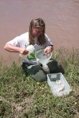
Sample Collection
Filtration for dissolved analysis, if desired, usually occurs during or immediately after sample collection. Samples can be frozen or chemically preserved. Equipment type and lab environment can affect phosphorus analysis, so extra care must be taken. Preparation of equipment used in phosphorus collection and analysis is strict and must be adhered to minimize contamination and sample error.
Acid Hydrolysis and Digestion
Digestions are used to estimate the total phosphorus and total organic phosphorus fractions (by subtraction). There are three principal digestion techniques: perchloric, nitric acid-sulfuric acid, and persulfate. Perchloric acid digestion is recommended only for the most difficult samples (e.g., sediments) and is time-consuming and severe. Nitric acid-sulfuric acid digestion is appropriate for most samples. Persulfate digestion is the simplest technique and should be checked against the other two for comparability.
Acid Hydrolysis
Acid hydrolysis is used for measuring the acid-hydrolyzable fraction and is defined as the difference between the concentrations in an untreated sample (reactive phosphorus) and one treated with mild acid. It includes condensed phosphates and potentially some organic phosphate compounds. This method involves acidifying a sample with sulfuric and nitric acids followed with gentle boiling. The orthophosphate liberated is then measured using one of the colorimetric methods.
Perchloric Acid Digestion
This fairly intense procedure involves acidifying a sample with nitric acid and then digesting the sample in a solution of nitric acid and perchloric acid. This is then neutralized with sodium hydroxide. Orthophosphate is then measured using one of the colorimetric methods.
Sulfuric Acid-Nitric Acid Digestion
This method uses a digestion rack much like those used for micro-Kjeldahl nitrogen determination. In this approach, sulfuric and nitric acids are added to a sample and digested. The orthophosphate liberated is then measured using one of the colorimetric methods.
Persulfate Digestion
In this approach, persulfate is added to a pH-adjusted sample and boiled for a set period of time. The orthophosphate liberated is then measured using one of the colorimetric methods.
Colorimetric Methods for Phosphate
The colorimetric methods are fairly similar and depend principally on the range of concentrations desired. The vanadomolybdophosphoric acid method is used for phosphate concentrations between 1 and 20 mg P/L and the stannous chloride and ascorbic acid methods are used for ranges between 0.01 and 6 mg P/L. Extractions and longer cell paths may improve detection on the lower ranges. Ion chromatography and capillary ion electrophoresis methods can also be used for determining orthophosphate concentrations in undigested samples.
Vanadomolybdophosphoric Acid Method
The principle of this test is that ammonium molybdate reacts with orthophosphate under acidic conditions and in the presence of vanadium to form a yellow color, which is proportional to the concentration of phosphate in the sample. This color can then be measured with a colorimeter and the phosphate concentration of the sample estimated. Again, this method is generally recommended over the 1 to 20 mg P/L range.
Stannous Chloride Method
In this method, molybdophosphoric acid (formed by the reaction of orthophosphate with ammonium molybdate under acidic conditions) is reduced by stannous chloride to form a blue molybdenum color, which is proportional to the concentration of phosphate in the sample. This color can then be measured with a colorimeter and the phosphate concentration of the sample estimated. With long path cells, this method can measure phosphorus down to 0.007 mg P/L. An extraction step using separation with benzene-isobutanol can increase the sensitivity for low concentration samples.
Ascorbic Acid Method
In this method, ammonium molybdate and potassium antimonyl tartrate react with orthophosphate under acidic conditions to form phosphomolybdic acid which is reduced to a blue color solution by ascorbic acid. The blue color formed is proportional to the concentration of phosphate in the sample. This color can then be measured with a colorimeter and the phosphate concentration of the sample estimated. The method is accurate to 0.01 mg P/L with a 5 cm cell path length. An extraction step using separation with solvent can increase the sensitivity for low concentration samples. An automated version of this method exists (APHA 1999; Method 4500- P F), which follows the same principal as the manual method but uses continuous flow analytical machines that automate the process and can be used for analyzing samples in large batches. The automated method is applicable over the range of 0.001 to 10.0 mg P /L. Higher concentrations can be diluted.
Literature Cited
APHA. 1999. Standard Methods for the Examination of Water and Wastewater. 20th edition. American Public Health Association, Washington, DC.
Elser, J.J., M.E.S. Bracken, E.E. Cleland, D.S. Gruner, W.S. Harpole, H. Hillebrand, J.T. Ngai, E.W. Seabloom, J.B. Shurin, and J.E. Smith. 2007. Global analysis of nitrogen and phosphorus limitation of primary producers in freshwater, marine and terrestrial ecosystems. Ecology Letters 10:1135-1142.
Francoeur, S.N. 2001. Meta-analysis of lotic nutrient amendment experiments: detecting and quantifying subtle responses. Journal of the North American Benthological Society 20:358-368.
Wetzel, R.G. 2001. Limnology: Lake and River Ecosystems. 3rd edition. Academic Press, New York.
Wetzel, R.G. and G.E. Likens. 2000. Limnological Analyses. 3rd edition. Springer-Verlag, New York.
Phytoplankton
Phytoplankton is the assemblage of autotrophs found in the water column, including diatoms, green algae, cyanobacteria, dinoflagellates, and other algal taxa. The phytoplankton includes single celled as well as colonial and filamentous forms, and it includes both true phytoplankton as well as periphytic algae that have been dislodged from the benthos (tychoplankton), especially in rivers. In waterbodies with sufficient residence time where true phytoplankton can develop (e.g., lakes, estuaries, and large rivers), this assemblage is the focus of sampling for algal response to nutrients and is, therefore, important in nutrient criteria development. There are well established relationships between nutrient loading and phytoplankton biomass in lakes. In rivers, the relationships are often more variable than those for lakes.
As with periphyton, two basic attributes of phytoplankton are most often sampled: biomass and composition. Biomass is generally measured by filtering phytoplankton and weighing the resultant organic matter, extracting the chlorophyll to provide a relative estimate of algal abundance, or counting the number of algal cells and using a biovolume conversion to estimate biomass. Phytoplankton assemblage composition typically consists of preserving a representative sample of water and identifying the algal taxa to the lowest possible taxonomic level. Both biomass and composition can be measured from the same field samples, which are split into a subsample for biomass and one for assemblage composition.
Chlorophyll a (analysis discussed below) has become one of the most widely used response variables when determining nutrient impairment. The benefits of chlorophyll a as an indicator are its sensitivity to stressors, such as nutrients, and ease of monitoring. Higher concentrations of chlorophyll a are indicative of algal production, which is responsive to nutrient pollution. A weakness of chlorophyll a as a measure of phytoplankton biomass/production is the variability of cellular chlorophyll content.
While many phytoplankton species cause harm in the context of eutrophication, others produce toxins, which can have a serious impact on aquatic systems. Harmful algal blooms (HABs) form as the result of proliferation of toxic nuisance algae and can cause a negative impact to natural resources and human health. Recently, there has been a noticeable increase in problems associated with HABs. Impacts of these natural phenomena include human illness (or death) from contaminated seafood, marine mammal and seabird deaths, and extensive fish kills. Of particular concern in freshwaters are cyanotoxins produced by cyanobacteria or blue-green algae. Cyanobacteria are abundant in most surface water when conditions are favorable for algal blooms. Cyanotoxins include neurotoxins, hepatotoxins, and dermatoxins and may cause a wide range of symptoms in humans. Microcystins are known to cause liver and kidney damage and may have severe long-term effects. For more information on HABs, refer to Harmful Algal Blooms.
The following is a brief review of common methods. Interested readers are encouraged to examine the literature cited for more detailed methodologies and greater background information.
Sample Collection
Phytoplankton samples can be collected using quantitative or semi-quantitative methods. Quantitative methods consist of sampling a volume of water, usually with a sampling device that can isolate a known volume at a specific depth (e.g., Van Dorn, Niskin, Nansen, or Kemmerer Bottle). Another option is to use a long, straight tubular sampler, which allows the collection of a depth integrated sample, essentially a “core” of the water column that collects plankton over a range of depths.
Algal Biomass
Algal biomass refers to the mass of algal material within the phytoplankton. It can be measured gravimetrically (weighed), using chlorophyll extractions, or by converting cell count data to mass using biovolume conversions. Gravimetric measures rely on weighing the amount or organic matter within the phytoplankton. As it is generally prohibitive to separate algal and non-algal material for routine analysis, the mass (usually the mass after combustion called ash-free dry mass [AFDM]) can include substantial non-algal material, although this is generally more severe in lotic than lentic systems. Some people use AFDM to chlorophyll ratios to look at the proportion of non-algal material, but this is only an approximation. The content of chlorophyll per cell varies with a number of factors: including species, nutrient conditions, light condition, and temperature. Therefore, chlorophyll is not a direct measure of biomass. However, it has long been used as a relative measure of algal abundance. Cell biovolumes vary by taxa, their shapes, and a number of other factors affecting cellular composition. However, if quantitative genus or species level data are collected, then biovolume can generally be estimated by applying shape specific geometric volume conversions.
Ash-free dry mass (AFDM)
A subsample of the original phytoplankton sample is either weighed in pre-combusted and pre-weighed crucibles or weighed following filtration through appropriate pre-weighed and pre-combusted glass fiber filters (0.5-0.7 µm pore size). Crucibles and filters are then dried, weighed for dry mass, and then combusted to remove all organic matter (e.g., 500ºC) and re-weighed to estimate AFDM. Samples for AFDM can be field filtered or brought to the lab for processing there. Sample preservation for AFDM is not straightforward, but samples should be handled to limit respiratory loss of organic matter [e.g., placed on ice and frozen (-20 to -60°C) if there will be a delay in processing]. Consult the specific methods for more on sample preservation. Values are expressed as grams AFDM per unit volume.
Pigment analysis
A subsample of the phytoplankton sample is usually filtered onto glass fiber filters (0.5-0.7 µm pore size) and used for pigment analysis as an indicator of algal biomass. On average, chlorophyll constitutes 1.5 percent of the AFDM of algae, but the ratio of chlorophyll to cell biomass varies by taxa, so biomass estimates using this technique should be considered relative. The composition of photosynthetic pigments also varies by algal taxa, but chlorophyll a is the principal pigment used because it is the most common and abundant. Chlorophylls b and c and the carotenoids absorb light at different wavelengths and can be quantified as well, if desired.
Chlorophyll a degrades into different phaeopigments that absorb at the same wavelength as chlorophyll a. For this reason, chlorophyll concentration is usually measured in a sample after extraction, acidified to convert all the chlorophyll to phaeopigments, remeasured, and chlorophyll a concentration is determined by the difference. Chlorophyll a is historically and most commonly measured using spectrophotometry, although fluorometry is more sensitive and becoming more commonly used.
Chlorophyll and other photopigments must be extracted from algae to quantify biomass using pigment analysis. It is best to work in low light to avoid degradation. While a variety of extraction solvents exist, alkaline aqueous acetone is still the standard recommended method. Algae retained on glass fiber filters (0.5-0.7 µm pore size) are typically ground in aqueous acetone, allowed to extract for a period of time under refrigeration in the dark, and the ground filter solution is centrifuged to separate the filter from the pigments. Pigments are then decanted and measured directly either with spectrophotometry or fluorometry. The flourometric method is usually standardized using spectrophotometric measurement of a chlorophyll extract and while fluorometry is more sensitive it should give comparable estimates. Consult an appropriate methods source for details on the use of either of these detection methods, including appropriate detectors, wavelengths, etc.
Preservation of samples for chlorophyll is important. Filtration should occur as soon as possible and chlorophyll should be extracted from filters as soon as possible. Field filtration is ideal. Addition of magnesium carbonate either to the sample solution or on top of the filter after filtration has been advocated to reduce acidity, since acidity degrades chlorophyll. Filters that will not be analyzed immediately, should be folded in half, placed into labeled dark containers (e.g., wrapped in aluminum foil), and placed on ice or immediately frozen. Pigment samples may be frozen for a few days (at -20 to -60°C), but should be analyzed as soon as possible, since degradation of chlorophyll does occur.
Biovolume
Biovolume is determined by multiplying the number of each taxon identified in a sample by the average biovolume of that taxon, calculated using equations of geometric shapes most approximating the shape of each taxon, and summing these values across all the taxa in a sample. Equations for many different taxa have already been developed or general equations may be applied. This approach obviously requires more effort, since individual taxa must not only be counted but average dimensions may calculated for each as well (average of 20 individuals is recommended, APHA 1999). This method does, however, offer one of the more accurate measures of live algal biomass.
Algal Composition
The composition of the algal assemblage of phytoplankton can provide information about the physical and chemical environment. Unlike simple grab samples of water, the assemblages of algae integrate water quality conditions over long periods of time. Each taxon has specific optima for the wide variety of physical and chemical conditions to which phytoplankton are exposed, including sensitivities or tolerance to nutrients, acidity, temperature, oxygen, silt, etc. The average environmental conditions influence which taxa survive and thrive. As a result, a great deal of environmental information, including nutrient conditions, can be inferred from which algae are found in the phytoplankton. This approach is applied by paleolimnologists, who identify the diatoms found in sedimentary strata of lakes to infer historical, even ancient, lake environmental conditions based on this principle. The composition of algae is usually determined with microscopy, and most taxa can be identified to species by well-trained taxonomists.
Microscopy
Unfiltered phytplankton samples should be preserved. The preferred preservative is Lugol’s solution, but other optional preservatives include 2% M3 fixative, 4% buffered formalin, or 2% glutaraldehyde. Phytoplankton samples containing macroalgae can be homogenized with a tissue homogenizer and placed into a specific cell for viewing larger algal taxa [e.g., Sedgwick-Rafter (up to 200x) or Palmer-Maloney (up to 500x) cells]. These can be enumerated a number of ways, but it can be difficult to enumerate colonial or filamentous individuals. Magnification is limited with these cells, so microphytoplankton often cannot be identified accurately. Sedimentation chambers and inverted microscopes(500-600x) are ideal for identifying large and smaller cells together. In this approach, a known subsample of the homogenized sample is placed into a sedimentation chamber, where the algae settle. The chamber is then placed on an inverted microscope, where higher objectives may be used. Ocular grids may improve counting efficiency. For the highest magnification (1000x), upright microscopes with oil immersion lenses are required. These are typically used for small diatom analysis. For diatom analysis, it is necessary to remove organic matter that might otherwise interfere with identifying diatoms. This can be done with combustion or chemical oxidation of subsamples, followed by slide mounting with a suitable highly refractive medium to make permanent slides. Other options include membrane filtration followed by clearing of the membranes. Compound microscopy at 1000x under oil immersion is then used to identify diatoms to species. Again, use of ocular grids may increase counting efficiency considerably. From these samples, accurate identification of the resident phytoplankton assemblage can be made. When combined with autecological information for the different algal taxa, a number of inferences about the integrated physical and chemical conditions of a lake can be made.
Remote Sensing
Phytoplankton can also be assessed via remote sensing of chlorophyll a. Ocean color satellites are capable of detecting optical components, such as chlorophyll a, and their respective concentrations in the water column according to the wavelengths of light they individually reflect back to the sensor. The sensor measures the remotely sensed chlorophyll a (chlorophyllRSa) signal by detecting the water leaving radiance in selected wavelengths of light per unit area. The signal read by the sensor is then used to derive quantitative information on the substances in the water and their concentrations in the near surface layers.
Literature Cited
APHA. 1999. Standard Methods for the Examination of Water and Wastewater. 20th edition. American Public Health Association, Washington, DC.
Boyer, J.N., C.R. Kelble, P.B. Ortner, and D.T. Rudnick. 2009. Phytoplankton bloom status: Chlorophyll a biomass as an indicator of water quality condition in the southern estuaries of Florida, USA. Ecological Indicators 9 (6, Supplement 1):S56-S67.
Hillebrand, H., C.D. Durselen, D. Kirschtel, U. Pollingher, and T. Zohary. 1999. Biovolume calculation for pelagic and benthic microalgae. Journal of Phycology 35: 403-424.
USEPA. 2012. Technical Support Document for U.S. EPA’s Proposed Rule for Numeric Nutrient Criteria, Volume 2 Coastal Waters. U.S. Environmental Protection Agency, Washington, DC.
USEPA. 2012. Cyanobacteria and Cyanotoxins: Information for Drinking Water Systems. EPA-810F11001. U.S. Environmental Protection Agency, Washington, DC.
Wetzel, R.G. 2001. Limnology: Lake and River Ecosystems. 3rd edition. Academic Press, New York.
Wetzel, R.G. and G.E. Likens. 2000. Limnological Analyses. 3rd edition. Springer-Verlag, New York.
Additional Information
ASTM Water Testing Standards Exit
Aquatic Informatics Resources Exit - Aquatic Informatics, Inc. has compiled a series of resources relating to water quality monitoring including an ebook, white papers, webinars, and case studies.
EPA Clean Water Act Analytical Methods - EPA publishes laboratory analytical methods or test procedures that are used by industries and municipalities to analyze environmental samples that are required by regulations under the authority of the Clean Water Act.
EPA Wetlands Modules - EPA prepared these modules to give states and tribes "state-of-the-science" information that will help them develop biological assessment methods to evaluate both the overall ecological condition of wetlands and nutrient enrichment.
National Environmental Methods Index (NEMI) - A free, searchable clearinghouse of methods and procedures for both regulatory and non-regulatory monitoring purposes for water, sediment, air, and tissues.
USGS Water Quality Methods and Techniques - USGS provides links to compiled information on water quality sampling methods.
USGS Field Guide for Collecting and Processing Stream - Water Samples for the National Water-Quality Assessment Program - The USGS National Water-Quality Assessment (NAWQA) program includes extensive data-collection efforts to assess the quality of the United States’ streams. These studies require analyses of stream samples for major ions, nutrients, sediments, and organic contaminants. This field guide describes the standard procedures for collecting and processing the previously mentioned samples, as well as field analyses of conductivity, pH, alkalinity, and dissolved oxygen.