Training Module on the Application of Best Modeling Practices | Environmental Measurements and Modeling

Best Modeling Practices: Application

This module builds upon the fundamental concepts outlined in previous modules: Environmental Modeling 101 and The Model Life-cycle. This module explains the Model Application Stage; the final step of the model life-cycle.

Model Life-cycle:
The processes included when taking the conceptual understandings of an environmental process to a full analytical model is called the model life-cycle. The life-cycle is broken down into four stages: identification, development, evaluation, and application.

When a modelmodelA simplification of reality that is constructed to gain insights into select attributes of a physical, biological, economic, or social system. A formal representation of the behavior of system processes, often in mathematical or statistical terms. The basis can also be physical or conceptual. is used to inform the decision-making process, it is important to consider the application nicheapplication nicheThe set of conditions under which the use of a model is scientifically defensible. The identification of application niche is a key step during model development. Peer review should include an evaluation of application niche. An explicit statement of application niche helps decision makers to understand the limitations of the scientific basis of the model. of the model; which will help to determine if the model is appropriate for a particular application. Additionally, the project team should consider their goals and expectations of the model, defined earlier in the project.

The objectives of this module are to identify the best modeling practices and strategies related to:

Model transparency
Documentation
Modeling scenarios with multiple models
Model post-audit

The life-cycle of a model including development, evaluation, and application stages; modified from EPA (2009a).
(Click on image for a larger version)

Model Application

Models are applied for a variety of reasons including (EPA, 2009a):

Hindcasting - to diagnose and examine causes and precursor conditions of events that have taken place
Forecasting - to forecast outcomes and future events
Characterize systems that are too complex to be addressed empirically

Complex model applications could involve a collaborative effort between modelers and program staff to devise management scenarios that represent different regulatory alternatives. The model would be used to evaluate the effects of those management scenarios.

Some model applications may include trial-and-error model simulations, where model inputs are changed iteratively until a desired environmental condition is achieved (EPA, 2009a).

Overview of models: connecting the real world to a formula

Models are representations of the environment that can be used to inform regulation or management decisions. They are simplifications constructed to gain insights into select attributes of a physical, biological, economic, or social system.

Uncertainty

There are many types of uncertaintyuncertaintyThe unknown effects of parameters, variables, or relationships that cannot or have not been verified or estimated by measurement or experimentation. associated with environmental modeling, and some degree of uncertainty will always be present when models are used. The act of applying a model (to inform a decision) introduces its own component of model uncertainty. This uncertainty arises from the context in which the model is applied, referred to as the application niche.

Model Uncertainty:
A general type of uncertainty comprised of application niche uncertainty, model structure/framework uncertainty, and input/parameter uncertainty.

Additional Web Resources:

For further information on uncertainty please see:

Categories of Model Uncertainty (EPA, 2009a)

Application niche uncertainty – uncertainty attributed to the appropriateness of a model for use under a specific set of conditions (i.e. a model application scenario).
Structure/framework uncertainty – incomplete knowledge about factors that control the behavior of the system being modeled; limitations in spatial or temporal resolution; and simplifications of the system.
Input/data uncertainty – resulting from data measurement errors; inconsistencies between measured values and those used by the model; also includes parameter value uncertainty.

Best Practices

Before selecting a model, the research team should have identified a specific scenario that could be informed from the application of a model. The characteristics and definition of each model’s application niche should clearly identify the suitable scenarios for future use of the model.

Application of a model to scenarios outside the bounds of its application niche is not recommended and may require an in-depth analysis of whether the model is truly appropriate for an application in the new context.

When parameterparameterA value used to numerically describe a population of values, e.g., the mean and standard deviation; or a value used to describe a dose-response curve, e.g., the intercept and the slope of a linear dose-response. calibrationcalibrationThe process of adjusting model parameters within physically defensible ranges until the resulting predictions give the best possible fit to the observed data. In some disciplines, calibration is also referred to as "parameter estimation". is specific to a modeling scenario, the subsequent application of that model outside of that scenario may result in erroneous predictions. For example, a threshold for health effects may exist at exposure levels below those covered by a particular epidemiological study. If that study is used in modeling health effects at those lower levels (and it is assumed that the level of response seen in the study holds for lower levels of exposure), then disease incidence may be overestimated (EPA, 2009b).

A Modeling Caveat

Extrapolation - is a process that uses assumptions about fundamental causes underlying the observed phenomena in order to project beyond the range of the data. In general, extrapolation is not considered a reliable process for prediction; however, there are situations where it may be necessary and useful (EPA, 2009a).

Resolution – Selection of spatial or temporal resolution (i.e., grid size) typically reflects a balance between a desired level of precision and resources required to model the system. If the resolution selected is too small, then key patterns of behavior reflected in the smaller step size may be missed altogether, or the behavior of the system may be misrepresented. (EPA, 2009b)

Case Study

Modeling the Risk of Lead Exposure in Children (EPA, 2007)

In this hypothetical scenario, data from four households with children are used to predict the risk of lead exposure. It is assumed that residents of each household are exposed to lead-contaminated soil. All other parameters are set to default values.

The selection of four houses is for illustration purposes only; a reliable estimate of neighborhood risk would require more than four houses. The probability density of lead concentration in the childrens’ blood (PbB) for the four houses is shown in Figure 1 and the interpreted results in Table 1.

The sum of the risks for these four houses 0.106% + 0.736% + 16.729% + 40.534% = 58.105%. That is, 0.581 children are expected to have blood lead concentrations (PbB) exceeding 10 µg/dL, or an average risk for a child living in this neighborhood would be 58.1%/4=14.5%.

The risk at two of the residences (houses 3 and 4) in the neighborhood is above the EPA’s Office of Solid Waste and Emergency Response specified level of protectiveness which aims to limit exposure to PbS levels such that a typical child or a group of similarly exposed children would have an estimated risk of no more than 5 percent exceeding the PbB level of concern (typically 10 µg/dL).

Figure 1. Probability density of blood lead in the hypothetical houses 1 to 4 (EPA, 2007).

Table 1

	House Number	PbS Concentration (µg/g)	PbD Concentration (µg/g)	Probability of exceeding 10 µg/dL
	1	250	47.5^A 0.	106
	2	250	185^B 0.	736
	3	1000	160^A 1	6.729
	4	1000	710^B 4	0.534
Risk from all houses 1-4:	58.105

^A Calculated using multiple source analysis and an MSD of 0.15
^B Calculated using multiple source analysis and an MSD of 0.70

Predicted risk of lead exposure in children with the IEUBKwin Model (EPA, 2007). Soil (PbS) and dust (PbD) concentrations of lead from each house are also shown. IEUBK Home Page.

Model Transparency

TransparencyTransparencyThe clarity and completeness with which data, assumptions and methods of analysis are documented. Experimental replication is possible when information about modeling processes is properly and adequately communicated. refers to the need for stakeholders, model output users, and members of the public to comprehend the essential workings of the model and its outputs (NRC, 2007).

Model transparency is an attractive attribute of models because it:

Enables effective communication between modelers, decision makers, and public
Allows models to be used reasonable and effectively in regulatory decision
Provides sufficient documentation
Allows for enhanced peer review

Model transparency is achieved when the modeling processes are documented with clarity and completeness at an appropriate level of detail. When models are transparent, they can be used reasonably and effectively in a regulatory decision. (EPA, 2009a).

An illustration of models as the 'black box' components of the scientific process. Models are often referred to as the ‘black box’ component of the scientific process. That is, the life-cycle of the model is often not transparent to decision makers, stakeholders, or the courts. Through an objective of overall transparency, model development teams can aim to make the model more transparent to stakeholder and user groups (Pascual, 2004).

Documentation

Documenting the decisions, assumptions, evaluation criteria, and other traits of a model is an important contribution to the model’s overall transparency.

Proper documentation provides a record of critical decisions and their justifications (NRC, 2007). Model documentation can often include an evaluation plan, a database of suitable data, a registry of model versions, or a user’s manual.

Additional Web Resources:

The topic of model documentation (an important component of a complete QA plan) is discussed in other modules as well:

Best Modeling Practices: Model Development

A discussion of the importance of model documentation in light of legal challenges, is included in another module:

Legal Aspects of Environmental Modeling

Key Aspects of a Model That Should be Documented (EPA, 2009a)

Data Quality Objectives**
Results **
Management Objectives
Conceptual Model
Choice of technical approach
Parameter Estimation
Uncertainty / Error
Conclusions of the analysis
Recommendations for additional analysis, if necessary
**Specific Recommendations

Communication

The modeling process should effectively communicate uncertainty to anyone interested in the model results. All technical information should be documented in a manner that decision makers and stakeholders can readily interpret and understand.

In addition to the results, the conclusions and other key points of the modeling project should be clearly communicated to decision makers. The challenge is to characterize the essential information for decision makers, while also providing them information about the modeling process and its limitations.

Decision makers should have sufficient insight into the model framework and its underlying assumptions to be able to apply model results appropriately. This is consistent with quality assurance planning practices for data quality that assert that technical reports must discuss the data quality and any limitations with respect to their intended use (EPA, 2000b).

Recommendations for Improving the Clarity of Modeling Communications (EPA, 2000c)

Be as brief as possible while still providing all necessary details.
Use plain language that modelers, policy makers, and the informed lay person can understand.
Avoid jargon and excessively technical language.
Define specialized terms upon first use.
Provide the model equations.
Use clear and appropriate methods to efficiently display mathematical relationships.
Describe quantitative outputs clearly.
Use understandable tables and graphics to present technical data

Best Practices

Documentation throughout the life-cycle of a model can support transparency objectives and help modelers use and improve the model in future model applications. Documentation should include any significant modifications to the assumptions and purpose(s) of the model (NRC, 2007).

Others have suggested the inclusion of stakeholders throughout the modeling life-cycle (especially during the Development Stage) as means for increasing transparency (EPA, 2008; Voinov and Bousquet, 2010).

Additional Resource:

An example of model documentation:

AQUATOX (Release 3): Modeling Environmental Fate and Ecological Effects in Aquatic Ecosystems Volume 2: Technical Documentation. (339 pp, 7.9 MB, About PDF) 2009. EPA-823-R-09-004.US Environmental Protection Agency. Washington, DC. Office of Water.

Attributes That Foster Transparency in Models (NRC, 2007)

Models should:

Be well documented
Address a specific concern
Be usable by decision makers and implementers
Be understandable by parties involved (e.g. decision makers; stakeholders; implementers)

Model Selection

A significant challenge for model applications is selecting an existing model to inform the decision making process (e.g. model selection during the development of a TMDLTMDLCalculation of the maximum amount of a pollutant that a waterbody can receive and still meet water quality standards and an allocation of that amount to the pollutant's source. for an impaired body of water); rather than developing a new model.

Model selection can involve qualitative and/or quantitative approaches. Under either approach, the team should have defined a clear description of the modeling scenario. The selection criteria should be chosen before the selection process and appropriately documented. The team should also consider (EPA, 2009a):

Whether the model’s complexity is appropriate for the problem at hand?
Do the quality and quantity of the data support the choice of model?
Does the model framework reflect all the relevant components of the conceptual model?
Has the model code been developed and verified?

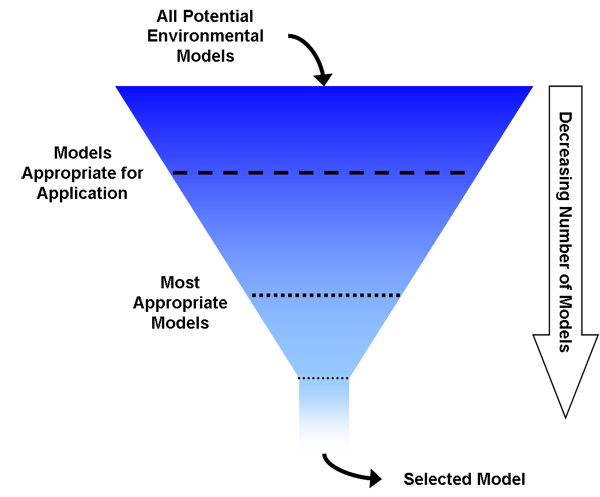
During a model selection process, all potential environmental models are examined to determine to (a) the most appropriate models and (b) the selected model(s). (Click on image for a larger version)

Qualitative Methods

Comparing qualitative attributes of a group of suitable models can help guide the selection of an appropriate model for a given application. Traits that could be compared are shown in the adjacent panel (EPA, 1995; 1997; Snowling and Kramer, 2001).

An example of a qualitative comparison is modified from EPA (1991). This review was limited to models that directly simulate water quality.

Additional Web Resources:

Qualitative traits of models that can be compared for Model Selection

Summary of modeling capabilities
Availability (proprietary vs. public domain)
Prior application / Traditional use / Degree of Acceptance
Requirements (e.g. staff, computer resources, input data, programming, etc.)
Output form and content (resolution)
Ease of application (sources, support, documentation)
Operating costs
Selected features relevant to application scenario
Theoretical basis of the model
Relative degree of model output uncertainty
Sensitivity (to input variability and uncertainty)
Complexity (level of aggregation; spatial and temporal scales)
Compatibility (if input/output linked to other models)
Reliability of model and code (peer review)

Quantitative Methods

During the development phase of an air quality dispersion model and in subsequent upgrades, model performance is constantly evaluated. These evaluations generally compare simulation results using simple methods that do not account for the fact that models only predict a portion of the variability seen in the observations.

The U.S. Environmental Protection Agency (EPA) developed a standard that has been adopted by ASTM International (formerly American Society for Testing and Materials), designation D 6589–00 for Statistical Evaluation of Atmospheric Dispersion Model Performance.

The statistical methods outlined in that report (similar to those in the adjacent panel) are not meant to be exhaustive. A few well-chosen simple-to-understand metrics can provide adequate evaluation of model performance (ASTM, 2000).

Deviance Measures Between Modeled (P) and Observed/Measured (O) Values

From Janssen and Heuberger (1995) n = number of observations.(Click on the formula images for a larger version.)

Average Error:

Modeling Efficiency:

Modeling efficiency formula.

Mean Square Error:

Mean Square Error formula.

Mean Absolute Error:

Root Mean Square Error:

Root Mean Square Error formula.

Multiple Models

In some model applications, a group of models may be appropriate for a certain decision making need. Applying multiple models, or multiple versions of a single model, is sometimes called ensemble modeling. For example, several meteorlogy models, each with its own strengths and weaknesses, might be applied for weather forecasting.

Similarly, stakeholders may suggest the use of alternative models to produce alternative risk assessments (e.g. CARES pesticide exposure model developed by industry).

Additional Web Resource:

Registry of EPA Applications, Models and Databases (READ)

Additional Resource:

Evaluation of Sediment Transport Models and Comparative Application of Two Watershed Models (PDF)(81 pp, 1.6 MB, About PDF). 2003. EPA-600-R-03-139. US Environmental Protection Agency. Cincinnati, OH. Office of Research and Development.

Ensemble Modeling: Case Study

A model is simplification of the system it represents. Therefore, running alternate versions of the same model can provide a probability of an expected outcome, rather than a single estimate. The alternate versions of the model may represent structural or parameter differences (e.g. Pinder et al., 2009).

Applying multiple models (of varying complexities) may provide insight into how sensitive the results are to different modeling choices and how much trust to put in the results from any one model (NRC, 2007). However, resource limitations or regulatory time constraints may limit the capacity to fully evaluate all the possible alternative models.

In this example, alternate versions of the CMAQ model are used to simulate how ozone concentrations change in relation to changes in input parameters. The ensemble of model estimates was shown to have a high level of skill and improved resolution and sharpness (Pinder et al, 2009).

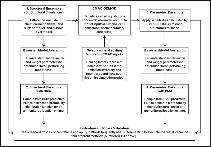
Ensemble Modeling: An example of the methodology for using an ensemble of models to produce a probabilistic outcome. Image adapted from Foley et al. (2008). (Click on image for a larger version)

The Model Post-Audit

Model corroboration demonstrates how well a model corresponds to measured values or observations of the real system. A model post-audit assesses the ability of the model to predict future conditions (EPA, 2009a). Post-audits are designed to evaluate the accuracy of model predictions, by comparing forecasts to actual observations (EPA, 1992; Tiedeman and Hill, 2007).

After a model has been used in decision support or applied, post-auditing would involve monitoring the modeled system to see if the desired (perhaps predicted) outcome was achieved.

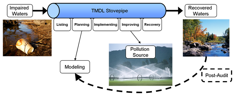
In this example, modeling was used to help develop a management plan forrecovering impaired waters by establishing Total Maximum Daily Loads (TMDLs) of a pollutant that a water body can receive and still safely meet water quality standards. During implementation of the TMDL, pollution sources were identified and regulated. The outcome (i.e. recovered water) is then compared to the predictions of the model.(Click on image for a larger version)

Best Practices

Post-auditing of all models is not feasible due to resource constraints, but targeted audits of commonly used models may provide valuable information for improving model frameworks and/or model parameter estimates.

In its review of the TMDL program, the NRC recommended that EPA implement audits by selectively targeting "some post-implementation TMDL compliance monitoring for verification data collection to assess model prediction error" (NRC, 2001).

The post-audit should also evaluate how effectively the model development and use process engaged decision makers and other stakeholders (Manno et al., 2008).

Post-audits can be used to identify the following types of model errors (Tiedeman and Hill, 2007)

Incorrect model parameter values that reasonably calibrate the model but that produce inaccurate predictions
Errors in the system conceptualization such as incorrect locations of system boundaries and inappropriate representation of flow and transport processes
Incorrect assumptions about the model calibration period being representative of the predictive period

Case Study: A Regional Air Quality Model

The U.S. Environmental Protection Agency’s NOx SIP Call required substantial reductions in NOx emissions from power plants in the eastern U.S.; with the emission controls being implemented during 2003 through May 31, 2004.

Since air quality models (e.g. CMAQ) are applied in order to estimate how ambient concentrations will change due to possible emission control strategies, the NOx SIP Call was identified an excellent opportunity to evaluate a model’s ability to simulate ozone (O₃) response to known and quantifiable observed O₃ changes.

The figure below provides an example from this prototype modeling study where changes in maximum 8-hour O₃ are compared from the summer 2005 period after the NOx controls to the summer 2002 before the NOx emission reductions occurred.

These results revealed model underestimation of O₃ decreases as compared to observations, especially in the northeastern states at extended downwind distances from the Ohio River Valley source region. This may be attributed to an underestimation of NOx emission reductions or a dampened chemical response in the model to those emission changes, or other factors.

Adapted from:
EPA's Dynamic Evaluation of a Regional Air Quality Model webpage

CMAQ model simulation results. CMAQ model simulation results were evaluated before and after major reductions in nitrogen oxides (NOx) emissions. Adapted from Gilliland et al. (2008).

Summary

Proper documentation throughout the model life-cycle will help to increase overall transparency.
The objective of transparency is to enable communication between modelers, decision makers, and the public. Models can be used reasonably and effectively in a regulatory decision when they are transparent (EPA, 2009a).
Models should be applied within their application niche.
Selecting an appropriate model for a specific application relies upon qualitative and quantitative measures. However, in some instances, it may be appropriate to apply multiple models and evaluate them collectively.
Model selection should be a transparent process that includes modelers, stakeholders and decision makers.
Ensemble modeling, when feasible, is a useful approach to include uncertainty estimates with deterministic models.
Post-audits are designed to evaluate the accuracy of model predictions by comparing forecasts to actual observations (EPA, 1992; Tiedeman and Hill, 2007).
Post-audits close the loop of the model life-cycle. Information gained during a post-audit can be used to further develop or update the model

You Have Reached the End of the Best Modeling Practices - Application Training Module

Check Done Icon

From here you can:

Continue exploring this module by navigating the tabs and sub tabs
Return to the Training Module Homepage
Continue on to another module:

You can also access the Guidance Document on the Development, Evaluation and Application of Environmental Models, March, 2009.

References

Andersen, P. F. and S. Lu. 2003. A Post Audit of a Model-Designed Ground Water Extraction System. Ground Water 41(2): 212-218.
ASTM. 2000. Standard Guide for Statistical Evaluation of Atmospheric Dispersion Model Performance. D 6589 – 05 West Conshohocken, PA. ASTM International.
EPA (US Environmental Protection Agency). 1991. Modeling of Nonpoint Source Water Quality in Urban and Non-urban Areas. EPA-600-3-91-039. Athens, GA. Office of Research and Development.
EPA (United States Environmental Protection Agency). 1992. Technical Guidance Manual for Performing Waste Load Allocations Book III: Estuaries Part 4: Critical Review Of Coastal Embayment And Estuarine Waste Load Allocation Modeling. EPA-823-R-92-005. Washington, D.C. Office of Water.
EPA (US Environmental Protection Agency). 1995. Technical Guidance Manual for Developing Total Maximum Daily Loads. Book II: Streams and Rivers Part 1: Biochemical Oxygen Demand/Dissolved Oxygen and Nutrients/Eutrophication. EPA 823-B-95-007. Washington, DC. Office of Water.
EPA (U.S. Environmental Protection Agency). 1997. Guiding Principles for Monte Carlo Analysis. EPA-630-R-97-001. Washington, DC. Risk Assessment Forum.
EPA (US Environmental Protection Agency). 2000a. Guidance for the Data Quality Objectives Process EPA QA/G-4. EPA/600/R-96/055. Washington, DC. Office of Research and Development.
EPA (US Environmental Protection Agency). 2000b. EPA Quality Manual for Environmental Program (PDF) (63 pp, 373 K, About PDF). CIO-2105-P-01-0. Washington, DC. Office of Environmental Information.
EPA (U.S. Environmental Protection Agency). 2000c. Risk Characterization Handbook. EPA-100-B-00-002. Washington, DC. Science Policy Council.
EPA (US Environmental Protection Agency). 2007. User’s Guide for the Integrated Exposure Uptake Biokinetic Model for Lead in Children (IEUBK) Windows® (PDF). (59 pp, 473 K, About PDF) 540-K-01-005 Office of Superfund Remediation and Technology Innovation
EPA (US Environmental Protection Agency). 2008. Integrated Modeling for Integrated Environmental Decision Making. EPA-100-R-08-010. Washington, DC. Office of the Science Advisor.
EPA (US Environmental Protection Agency). 2009a. Guidance on the Development, Evaluation, and Application of Environmental Models. EPA/100/K-09/003. Washington, DC. Office of the Science Advisor.

References (Continued)

EPA (US Environmental Protection Agency). 2009b. Using Probabilistic Methods to Enhance the Role of Risk Analysis in Decision-Making With Case Study Examples. DRAFT. EPA/100/R-09/001 Washington, DC. Risk Assessment Forum.
Foley, K. M., R.W. Pinder, S.L. Napelenok, and H.C. Frey. Probabilistic Estimates of Ozone Concentrations from an Ensemble of CMAQ Simulations, poster for Models-3 Users' Conference, Chapel Hill, October 2008.
Gilliland, A.B., C. Hogrefe, R.W. Pinder, J.M. Godowitch, K.L. Foley, S.T. Rao. Dynamic evaluation of regional air quality models: Assessing changes in O3 stemming from changes in emissions and meteorology. Atmospheric Environment,42, 5110-5123, 2008.
Janssen, P. H. M. and P. S. C. Heuberger 1995. Calibration of process-oriented models. Ecol. Model. 83(1-2): 55-66.
Manno, J., R. Smardon, J. V. DePinto, E. T. Cloyd and S. Del Granado. 2008. The Use of Models In Great Lakes Decision Making: An Interdisciplinary Synthesis Randolph G. Pack Environmental Institute, College of Environmental Science and Forestry. Occasional Paper 16.
NRC (National Research Council). 2001. Assessing the TMDL Approach to Water Quality Management. Washington, DC. National Academies Press.
NRC (National Research Council). 2007. Models in Environmental Regulatory Decision Making. Washington, DC. National Academies Press.
Pascual, P. 2004. Building The Black Box Out Of Plexiglass. Risk Policy Report 11(2): 3.
Pinder, R. W., R. C. Gilliam, K. W. Appel, S. L. Napelenok, K. M. Foley and A. B. Gilliland. 2009. Efficient Probabilistic Estimates of Surface Ozone Concentration Using an Ensemble of Model Configurations and Direct Sensitivity Calculations. Environ. Sci. Technol. 43(7): 2388-2393.
Snowling, S. D. and J. R. Kramer. 2001. Evaluating modelling uncertainty for model selection. Ecol. Model. 138(1-3): 17-30.
Tiedeman, C. R. and M. C. Hill. 2007. Model Calibration and Issues Related to Validation, Sensitivity Analysis, Post-audit, Uncertainty Evaluation and Assessment of Prediction Data Needs. In: Groundwater: Resource Evaluation, Augmentation, Contamination, Restoration, Modeling and Management. Ed. M. Thangarajan. Springer Netherlands. 237-282.
Voinov, A. and F. Bousquet. 2010. Modelling with stakeholders. Environ. Model. Software 25(11): 1268-1281.