Guidance for Using PRZM-GW in Drinking Water Exposure Assessments
PDF Version
Guidance for Using PRZM-GW in Drinking Water Exposure Assessments (20 pp, 622K, About PDF)
Memorandum (1 pp, 36K, About PDF)
October 15, 2012
Prepared by:
Reuben Baris; Michael Barrett, PhD; Rochelle F. H. Bohaty, PhD; Marietta Echeverria;
Philip Villanueva; James Wolf, PhD; Dirk Young, PhD
On this Page
- Appendix 1. Tier 1 Pre-implementation Analysis: A Comparative Evaluation of PRZM-GW 1.0 and SCI-GROW 2.3
Memorandum
December 11, 2012
SUBJECT: Approval of PRZM-GW for Use in Drinking Water Exposure Assessments
FROM: /s/ Donald Brady, Director, Environmental Fate and Effects Division (7507P), Office of Pesticide Programs
TO: Environmental Fate and Effects Division (7507P), Office of Pesticide Programs
The Pesticide Root Zone Model for GroundWater (PRZM-GW)1 is now available for standard use in screening (Tier I) and refined (Tier II) drinking water assessments. PRZM-GW is available on the share drive (G:\Models_Repository) and EFED's Water Models website. Guidance for using PRZM-GW is found in Attachments 1, 2 and 3.
During a one-year evaluation period, scientists should estimate Tier I drinking water concentrations using PRZM-GW and SCI-GROW (Screening Concentration in Groundwater). For Tier I assessments, the results from the model (either SCI-GROW or PRZM-GW) that estimates the highest EDWCs should be incorporated along with surface water EDWCs in the executive summary of the drinking water exposure assessments. For Tier II drinking water assessments, PRZM-GW should be used according to the attached user guidance. SCI-GROW is not used in Tier II drinking water assessments.
For questions concerning PRZM-GW, please contact the Water Quality Technical Team. For questions concerning installation, please contact Environmental Information and Services Branch (EISB).
Attachments:
Guidance for Using PRZM-GW in Drinking Water Exposure Assessments
Guidance for Selecting Input Parameters for Modeling Pesticide Concentrations in Groundwater Using the Pesticide Root Zone Model
Model and Scenario Development Guidance for Estimating Pesticide Concentrations in Groundwater Using the Pesticide Root Zone Model
Introduction
Under the auspices of the North American Free Trade Agreement (NAFTA), the Environmental Protection Agency's (EPA) Office of Pesticide Programs (OPP) and Canada's Pesticide Management Regulatory Authority (PMRA) completed a groundwater modeling harmonization project in 2012. After this project was completed, the two agencies issued a final report on the Identification and Evaluation of Existing Models for Estimating Environmental Pesticide Transport to Groundwater.1 In order to implement the final report, the Environmental Fate and Effects Division (EFED) in OPP developed a guidance document, which establishes a formal procedure for using the PRZM-GW (Pesticide Root Zone Model for GroundWater) as a screening-level and refined tool for risk assessment purposes. In general, PRZM-GW provides conservative estimates of pesticide concentrations in groundwater, but it also allows for region specific scenario development in cases where refined drinking water assessments are needed.2
The following components are included in the current guidance document for implementing the EPA-PMRA final report:
a summary of the groundwater conceptual model implemented in PRZM-GW;
a brief synopsis of the PRZM-GW evaluation; and
step-by-step instructions on how to use PRZM-GW in OPP tiered risk assessments (see the METHODS section of this document).
The document also contains guidance on interpreting PRZM-GW output data, characterizing the data for risk assessments, as well as strategies for refining drinking water assessments when needed. This guidance is under evaluation for one year, after which time it may be modified as needed.
1 Baris, R.; Barrett, M.; Bohaty, R.; Echeverria, M.; Kennedy, I.; Malis, G.; Wolf, J.; Young, D. Final Report: Identification and Evaluation of Existing Models for Estimating Environmental Pesticide Transport to Groundwater; Health Canada, U.S. Environmental Protection Agency, October 15, 2012.
2 U.S. Environmental Protection Agency. Federal Insecticide, Fungicide, and Rodenticide Act (FIFRA) Scientific Advisory Panel: N-Methyl Carbamate Pesticide Cumulative Risk Assessment: Pilot Cumulative Analysis, February 15-18, 2005 (a), 2005-01, Docket Number: OPP-2004-0405.
Background
After the passage of the Food Quality Protection Act (FQPA) of 1996, the EPA developed SCI-GROW (Screening Concentration in Groundwater) as a screening-level tool to estimate drinking water exposure concentrations in groundwater resulting from pesticide use (Barrett, 1997).3 As a screening tool, SCI-GROW provides conservative estimates of pesticides in groundwater, but it does not have the capability to consider variability in leaching potential of different soils, weather (including rainfall), cumulative yearly applications or depth to aquifer. If SCI-GROW-based assessment results indicate that pesticide concentrations in drinking water exceed levels of concern, the ability to refine the assessment is limited.
In 2004, OPP initiated an evaluation of advanced methods for estimating pesticide concentrations in groundwater as part of the cumulative risk assessment of carbamate pesticides. OPP consulted with the FIFRA Scientific Advisory Panel (SAP) twice in 2005 on the development of the groundwater conceptual model and the use of PRZM to implement the conceptual model.4, 5 Concurrently OPP and PMRA initiated a project under the auspices of the North America Free Trade Agreement (NAFTA) Technical Working Group on Pesticides to develop a harmonized approach to modeling pesticide concentrations in groundwater. The final NAFTA project report recommends PRZM-GW as the harmonized tool for assessing pesticide concentrations in groundwater. Included in the final report is a summary of the model evaluation, guidance for scenario development, and chemical input parameter guidance.
3 SCI-GROW is an empirical model based on a linear best fit through 13 single-application groundwater studies. These studies were typically two to three year studies. SCI-GROW is a screening level risk assessment tool that has been used by OPP to evaluate the effect of pesticide use on groundwater.
4 U.S. Environmental Protection Agency. Federal Insecticide, Fungicide, and Rodenticide Act (FIFRA) Scientific Advisory Panel: N-Methyl Carbamate Pesticide Cumulative Risk Assessment: Pilot Cumulative Analysis, February 15-18, 2005 (a), 2005-01, Docket Number: OPP-2004-0405.
5 U.S. Environmental Protection Agency. Federal Insecticide, Fungicide, and Rodenticide Act (FIFRA) Scientific Advisory Panel: Preliminary N-Methyl Carbamate Cumulative Risk Assessment, August 23-26, 2005 (b), 2005-04, Docket Number: OPP-2005-0172
Conceptual Model
Figure 1 depicts the general groundwater scenario concept for estimating pesticide concentrations in drinking water as implemented in PRZM-GW. This conceptual model is based on a rural drinking water well beneath an agricultural field (a high pesticide use area), which draws water from an unconfined, high water-table aquifer.
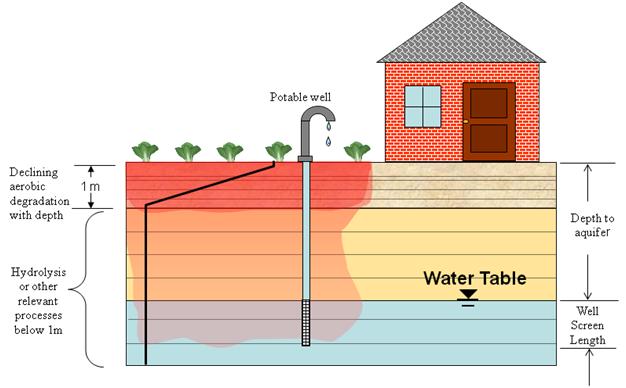
Figure 1
General Groundwater Scenario Concept for Estimating Pesticide Concentrations in Drinking Water
as Implemented in PRZM-GW
The depth of the well is site-specific (i.e., scenario specific). The well extends into a shallow unconfined aquifer and has a well-screen6 that starts at the top and continues down into the aquifer. The length of the well-screen represents the region of the aquifer where drinking water is collected. The well-screen length is well-specific and can be adjusted. Processes included in the conceptual model that influence pesticide transport through the soil profile include water flow, chemical specific dissipation and transportation parameters (i.e., degradation and sorption), and crop specific factors, including transpiration, pesticide interception and management practices.
6 A well-screen is a filtering device that allows groundwater from unconsolidated and semi-consolidated aquifers to enter the well while at the same time keeping the majority of sand and gravel out of the well.
PRZM-GW Evaluation
Monitoring Data Comparison
The conceptual model as implemented in PRZM-GW was assessed based on the performance of PRZM-GW as a screening tool7 for estimating pesticide concentrations in groundwater. The EDWCs generated using PRZM-GW 1.0 were compared to targeted and non-targeted groundwater monitoring data. (The results of this comparison are included in the NAFTA project final report1). The capabilities of the PRZM-GW model were assessed on both a national and site-specific basis. The analysis considered maximum predicted pesticide concentrations resulting from PRZM-GW simulation using six different scenarios8 specifically developed for the PRZM-GW model and high-end pesticide detections from selected monitoring studies: National Ambient Water Quality Assessment (NAWQA) Program, Acetochlor Registration Partnership (ARP) Midwest Corn Production Area (MwCPA) Program, National Alachlor Well-Water Survey (NAWWS) and a North Carolina Prospective Groundwater (PGW) Study. 1 The locations of the six standard PRZM-GW scenarios are shown in Figure 2.
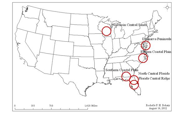
Figure 2
PRZM-GW Specific Groundwater Scenario Locations
In summary, the evaluation showed that PRZM-GW EDWCs (maximum concentration of the six standard scenarios) were usually greater than the observed concentrations. In some cases, over predictions were as high as 1000x. It was concluded that the overestimations were likely the result of the limitations of the comparison of the simulation data and the monitoring dataset. For example, the monitoring samples may have been taken in areas that did not reflect high use sites for a given pesticide; the wells sampled may not represent vulnerable groundwater resources and thus are not representative of the conceptual model or the scenarios used in the PRZM-GW simulations; or the actual field use rates, application dates or application treatment intervals were different from those modeled. Overestimations may also result from the use of conservative model input parameters (3x aerobic soil metabolism half-life value when only one aerobic soil metabolism study is available).
In a few cases, PRZM-GW underestimated pesticide concentrations observed in groundwater. While more analysis may provide additional insight, it was concluded that these underestimations may be the result of pH dependent hydrolysis, high variability of the degradation rates under the actual environmental conditions, or transport mechanisms (e.g., preferential flow or macroparticle transport) not considered in the conceptual model (Figure 1) as implemented in PRZM-GW. The evaluation indicates that PRZM-GW can underestimate pesticide concentrations with high sorption coefficients (i.e., Koc > 1000 mL/goc) and low persistence (i.e., soil half-life < 30 days). In addition, there are a few instances where PRZM-GW estimated concentrations of low-sorbing chemicals (Koc) were less than monitoring data. The final report describes the conditions under which underestimation may occur. When PRZM-GW simulations are designed to reflect site-specific parameters, the predicted concentrations are similar (within an order of magnitude) to the monitoring concentrations.
7 An effective groundwater screening tool, works to simulate concentrations greater than those observed in the vast majority of drinking water wells. In a non-targeted context, an effective screen provides concentrations that are greater than those observed in monitoring studies.
8 Florida Citrus, Florida Potato, Wisconsin Corn, Georgia Peanuts, North Carolina Cotton, and Delmarva Sweet Corn
SCI-GROW Comparison
The performance of PRZM-GW as a screening-level Tier I risk assessment tool was compared to performance of the current method employed to estimate pesticide concentrations in ground water (i.e., SCI-GROW). For this analysis, both PRZM-GW 1.0 and SCI-GROW 2.3 estimated pesticide concentrations were compared to groundwater concentrations for 66 chemicals included in the NAWQA dataset.
In general, PRZM-GW EDWCs were higher than SCI-GROW EDWCs for the suite of chemicals included in the evaluation (Figure A.1). This difference may be explained by the narrow range of studies that were evaluated in the 13 PGW studies that formed the basis of SCI-GROW. The PGW studies investigated the leaching potential of chemicals with Koc and half-life values that ranged from 32-180 mL/goc and from 13-1000 days, respectively, and did not capture some of the fate parameters for the evaluated chemicals that fell outside this range. In addition, the PGW studies only considered one year of pesticide application, whereas PRZM-GW simulations included in the evaluation considered multiple years (up to 100 years) of repeated pesticide application.
On a few occasions, PRZM-GW EDWCs were lower than SCI-GROW EDWCs for the chemicals included in the evaluation (Figure A.1). In general, these results were observed for highly sorbing (Koc >10,000 mL/goc) chemicals for which the underestimations were likely the result of transport mechanisms (e.g., preferential flow or macroparticle transport). These factors were not considered in the groundwater conceptual model (Figure 1) implemented in PRZM-GW and the resulting simulations, but they were captured by the lower bound concentration limit (0.006 ppb per lb ai/a applied) included in SCI-GROW.
Evaluation Summary
After a complete evaluation, PRZM-GW was determined to be an effective tool for establishing upper bound pesticide concentrations in groundwater for national as well as site-specific assessments. As such, it could be used as a screening model for Tier I as well as Tier II drinking water assessments. Including SCI-GROW EDWCs in Tier I drinking water assessment was also shown to be an adequate strategy (Table A.1) for capturing the potential for some chemicals to be transported into drinking water wells by mechanisms not included in the groundwater conceptual model (Figure 1). During the one-year evaluation period, both PRZM-GW and SCI-GROW EDWCs should be reported in drinking water exposure assessments as discussed below.
OPP Tiered Groundwater Exposure Assessments
Tier 1
A summary of the process for completing a Tier 1 groundwater assessment is provided in Figure 3. Step-by-step instructions on how to complete this process are provided below.
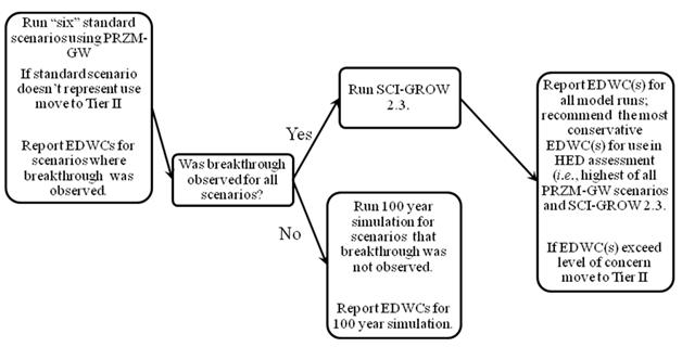
Figure 3
Tier 1 Groundwater Exposure Assessment Process Diagram
Standard Tier I Groundwater Assessment: Running PRZM-GW
Step 1: Starting PRZM-GW
To open the PRZM-GW window, click on the "PRZM GW.exe" icon.
Step 2: Prepare Pesticide Specific Parameters for Model Runs
Under the first tab labeled "pesticide," complete (Figure 4) the appropriate fields, including chemical name and descriptive information, followed by the hydrolysis half-life, aerobic soil metabolism half-life and sorption coefficient. The PRZM-GW specific input parameter guidance has been developed and is included as Attachment 1 of the final report;9 however, it is the responsibility of the model user to follow the current input parameter guidance for PRZM-GW on the date the model runs are completed.
Select the number of applications, corresponding application dates (absolute and relative), rates, methods, and annual application retreatment based on the pesticide use label. Descriptions of each of the parameters are provided in the GUI help file under User Guidance. For Tier 1 assessments, the maximum label rates and minimum retreatment intervals should be used, and the annual application retreatment should be left at the default value of one (or once every year).
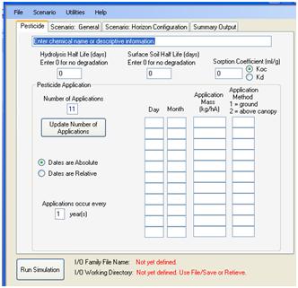
Figure 4.
Screen Shot of PRZM-GW Pesticide Tab
Table 1 should be completed and included in individual drinking water assessments to document input parameter selections for PRZM-GW model runs. It is the responsibility of the user to conduct modeling according to the current input parameter guidance. For specific cases, where deviation from the guidance is appropriate, the model user should document the rationale for each deviation from the current guidance. (Additional guidance can be found in the Tier 2 section of this document). If additional guidance is desired, OPP model users may consult with the EFED's Water Quality Technology Team (WQTT).
Table 1
PRZM-GW Input ParametersParameter (units) Input Value Data Source Comments Application Rate Number of Applications Application Date(s) Annual Application Retreatment Hydrolysis Half-life (days) Soil Metabolism Half-life (days) Koc (mL/goc) Since hydrolysis is generally the only transformation pathway considered at soil depths greater than one meter, it can have a large impact on the PRZM-GW EDWCs. A chemical may be assumed to be stable to hydrolysis based on minimal transformation in the guideline hydrolysis study (OCSPP 835.2120); however, reevaluation of the hydrolysis study may be completed for such chemicals. If reevaluation of the study shows that a small but statistically significant amount of hydrolysis was observed during the course of the study, a hydrolysis rate should be recalculated along with the corresponding half-life. In this case, including the hydrolysis rate, even if very slow (extrapolation well beyond the study duration), provides better pesticide estimation compared to monitoring data than assuming the chemical is stable. Characterization (e.g., examination of the upper bound of the hydrolysis rate) of the influence of hydrolysis on the PRZM-GW simulation results should be reported.
To save the chemical inputs, click file and select save. Point the browser to the desired folder destination to save a computer file.
Previously saved chemical files can be loaded by clicking "File" and selecting "Retrieve" (pointing the browser to the desired chemical file). The file will need to be resaved following any changes.
9 Baris, R.; Barrett, M.; Bohaty, R.; Echeverria, M.; Kennedy, I.; Malis, G.; Wolf, J.; Young, D. PRZM-GW Input Parameter Guidance; Health Canada, U.S. Environmental Protection Agency, October 12, 2012.
Step 3: Save Pesticide Specific Parameters for Model Runs
Click on "File" and select "Save." Create a file name and save the file to the desired directory.
Step 4: Select Scenario Parameters for Model Runs
Six standard scenarios, which represent regions known to have vulnerable groundwater supplies, have been developed for use with PRZM-GW: Wisconsin Central Sands, New Jersey/Delaware Delmarva Coast, Florida Sands, Florida Central Ridge, and North Carolina Sands. Details on the individual scenarios can be viewed under the second and third tabs, "Scenario: General" and "Scenario: Horizon Configuration," respectively. To load a scenario, click on "Scenario" at the top of the GUI and then select "Load Scenario." Scenarios current as of the date of this memo are noted as June 2012; however, it is the responsibility of the model user to use current scenarios as of the model run date.
For Tier I assessments, all six scenarios should be run for national scale pesticide assessments. However, if the use is restricted by geography, the user should identify the best representative surrogate scenario(s). In choosing an appropriate surrogate scenario, users should consider the location of each scenario as it relates to the pesticide use area and climatic conditions, including rainfall and soil hydrology as the primary selection criteria, followed by crop type (e.g., corn, cotton, cucurbits, etc.). When a surrogate scenario is used, the model user should document the rationale for using the surrogate scenario including a description and justification. If guidance is needed for selecting an appropriate surrogate scenario, OPP model users should consult with EFEDs Water Quality Technology Team (WQTT). For specific cases, when a suitable standard scenario is not available, a new scenario can be developed. (See the Tier 2 section Refinement Strategy 1 included in this document).
Step 5: Running Groundwater Simulations and Viewing Results
Click on the fourth tab "Summary Output," and then click the "Run Simulation" button located in the bottom left corner of the GUI to run the simulation. ("Run Simulation" is visible in the screen shot shown in Figure 5a). The summary output contains a graph of the daily concentration values over the course of the simulation as shown in Figure 5b. This graph can be saved or copied to the computer clipboard, using the buttons in the middle of the GUI.
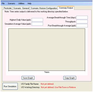
Figure 5a
Screen Shot of Summary Output Tab
(a) before simulation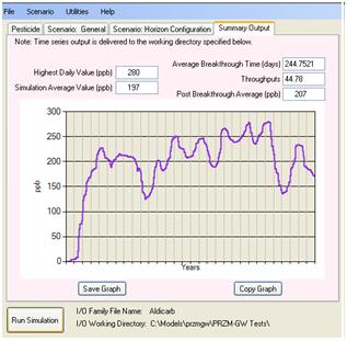
Figure 5b
Screen Shot of Summary Output Tab
(b) after simulation
The summary report includes the highest daily value, simulation average value, average simulation breakthrough time, throughputs, and post breakthrough average. These values are defined below.
Highest Daily Value: The highest daily concentration for the entire simulation reported in parts per billion (ppb, µg/L).
Simulation Average Value: The average concentration for the entire simulation reported in parts per billion (ppb, µg/L). This takes into account zero values (observed before breakthrough) in the calculated average concentration reported in parts per billion (ppb, µg/L).
Average Simulation Breakthrough Time: The number of days that it takes for the applied chemical to reach the aquifer.
Throughputs: The estimated pore volumes/retardation factor that occurs in the simulation.
If throughput value is less than one, see Step 6 to create a weather extended file for a 100-year simulation.
Post Breakthrough Average: The average concentration reported in parts per billion (ppb, µg/L) for the simulation after breakthrough; the time when the applied chemical reaches the aquifer.
All model output files are created in the same directory where the input file is saved after the model simulation is complete.
Step 6, if needed: Use of an Extended Weather File
If the "throughputs" value for a model run is less than one, modeling should be repeated with the appropriate extended weather file. An extended weather file contains the same weather as the standard 30-year weather file and allows the user to run the simulation for up to 100 years in order to observe breakthrough. To create an extended weather file, make sure the weather file to be extended is listed on the second tab "Scenario: General," then click on "Utilities." Next, select the "Create Extended Weather File" tool. The user will be asked in a popup window "Do you want to create an extended weather file?" To complete the process, click the "yes" button.
To run a PRZM-GW simulation with an extended weather file, select the "Select Weather" button on the second tab "Scenario: General." Point the browser to the "Metfiles" directory and select the appropriate extended weather file. All extended weather files are named using the weather station identification number, followed by the word "Extended" (e.g., W13781Extended.dvf).
Once an extended weather file has been created it will be saved with all the other weather files and a new extended weather file for that specific station will not need to be re-created for subsequent runs requiring an extended weather file for that station.
Step 7: Reporting Results in Drinking Water Assessments
For all drinking water assessments, a description of PRZM-GW should be included in the Drinking Water Exposure Modeling section. This information should include a description of the model, including version and version dates. The following example can be used:
Tier 1 groundwater estimated drinking water concentrations (EDWCs) for [insert chemical being assessed], resulting from its use on [insert crop uses being assessed] were derived with PRZM-GW (Pesticide Root Zone Model for Groundwater, version 1.0, August 31, 2012), using the GW-GUI (Graphical User Interface, version 1.0, August 31, 2012). PRZM-GW is a one-dimensional, finite-difference model that estimates the concentrations of pesticides in groundwater. It accounts for pesticide fate in the crop root zone by simulating pesticide transport and degradation through the soil profile after a pesticide is applied to an agricultural field. PRZM-GW permits the assessment of multiple years of pesticide application (up to 100 years) on a single site. Six standard scenarios, each representing a different region known to be vulnerable to groundwater contaminations, are available for use with PRZM-GW for risk assessment purposes. In PRZM-GW simulations, each of these standard scenarios was used. PRZM-GW output values represent pesticide concentrations in a vulnerable groundwater supply that is located directly beneath a rural agricultural field.
PRZM-GW simulation results should be included in drinking water exposure assessments by crop. The highest peak value should be reported for short-term exposure, while the post-breakthrough average should be reported for longer term exposures. In addition, the average simulation breakthrough time should be reported. An example table, which can be used to summarize the EDWCs for drinking water exposure assessment, is presented below (Table 2). The PRZM-GW derived EDWCs should be characterized as representing vulnerable drinking water supplies as described in the conceptual model section of this document. The results from the simulation that provides the highest EDWC should be incorporated with surface water EDWCs and highlighted in the executive summary of the drinking water exposure assessment.
Table 2
PRZM-GW Estimated Drinking Water Concentrations in Groundwater
Resulting from the Use of [insert chemical being assessed]Crop/Scenario Highest Daily Value
µg/LPost Breakthrough Average
µg/LAverage Simulation Breakthrough Time
days[Crop]/Tier I [Standard Scenario] [#] [#] [#] [Crop]/Tier I Standard Scenario [#] [#] [#] A percent cropped area (PCA) adjustment factor should not be applied to PRZM-GW model output data to generate estimated drinking water concentrations (EDWCs). The conceptual model for groundwater exposure, as implemented using PRZM-GW, represents pesticide concentrations in a vulnerable groundwater supply that is located directly beneath a single, rural agricultural field and assumes the entire field (zone of influence) is treated. The zone of influence does not represent an entire watershed.
Tier 2
A summary of the process for completing a Tier 2 groundwater exposure assessment is provided in Figure 6. Step-by-step instructions on how to complete this process are also provided in the refinement strategy sections below.
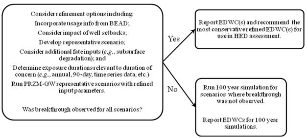
Figure 6
Tier II Groundwater Exposure Assessment Process Diagram
Standard Tier II Groundwater Assessment: Refinement Strategies
Refinement Strategy 1: Development of Representative Scenario
It may be necessary to develop a scenario that specifically represents a use site for which one of the standard scenarios is not a suitable surrogate. For example, a new scenario may be needed when mitigation measures prohibit the use of a given pesticide in areas known to be prone to groundwater contamination. Soil type and characteristics, weather data, and depth to aquifer are all refinements that can be included in a site-specific scenario. To ensure consistency in the development and use of crop scenarios, scenarios developed for use with PRZM-GW should follow the PRZM-GW Scenario Development Guidance10 and should be shared with EFED's WQTT before being used in an exposure assessment. All WQTT approved scenarios will be distributed to members of the WQTT for use in exposure assessments to ensure consistency within OPP.
10 Baris, R.; Barrett, M.; Bohaty, R.; Echeverria, M.; Wolf, J.; Young, D. PRZM-GW Scenario Development Guidance U.S. Environmental Protection Agency, October 15, 2012.
Refinement Strategy 2: Identify Pesticide Fate Parameters not Considered in the Tier 1 Simulations
There are several different chemical specific parameters that can be considered for refinement as well as additional subsurface transformation or adsorption processes. Consideration of additional subsurface transformation or sorption processes should be considered if data are available on relevant subsurface processes, including subsurface degradation and subsurface sorption.
For subsurface transformation, it should be noted that the field "Hydrolysis Half-Life" only considers transformation occurring in the aqueous phase, while the "Surface Soil Half-Life" considers both sorbed and aqueous phase transformation. OPP model users should consult EFED's Water Quality Technology Team (WQTT) before modifying these parameters to ensure the adequacy of the relevant data and the appropriate modification of the transformation rates. All changes should be described and characterized in the refined drinking water assessment. In addition, the influence of the modifications on the PRZM-GW simulation results should be reported in the assessment.
Refinement Strategy 3: Consideration of Annual Application Retreatment
If data are available [such as from the Biological and Economic Analysis Division (BEAD) or provided on the label] on the yearly reoccurrence of the pesticide applications, this information can be considered in model runs. To change the application reoccurrence, click on the "Pesticide" tab and change the field "Applications occur every "x" year(s)" to the appropriate value. The model user should document the rationale for changing the application reoccurrence in the refined drinking water assessment and discuss the impact on the PRZM-GW simulation results. The annual applications retreatment interval should be recommended as additional label language.
Refinement Strategy 4: Considerations of Well Setbacks
To account for the well setback distances specified on a pesticide label, a plug flow model can be used to simulate the additional travel time for a pesticide to reach a drinking water well from the point of application. Reductions in the expected concentration can be calculated in drinking water assessments using the plug flow approximation:5
C/C0 = exp((-L/v)k)
where:
C = concentration at well [mass/volume]
C0= concentration at point of application [mass/vol]
L = well setback distance [length]
v = lateral groundwater velocity [length/time] (e.g., 0.15 m/day)
k = degradation rate in aquifer [time-1]
Additional information of well setbacks is provided in the preliminary N-methyl carbamate cumulative assessment.4,5
-
Refinement Strategy 5: Exploring Exposure Durations That Are Representative of the Exposure Duration of Concern
The model output file will be saved in the same directory as the input file. The output file contains the daily distribution of pesticide concentrations, which can be provided for use in the Human Health Assessment.11 Additional post processing can be completed to develop exposure values that reflect the exposure duration of concern. Programs such as Excel, SigmaPlot, or R can be used for post processing of the data.
11 Guidance on Generating Drinking Water Distribution Files for HED's Dietary Risk Assessments, January 21, 2005.
Appendix 1
Tier 1 Pre-implementation Analysis:
A Comparative Evaluation of PRZM-GW 1.0 and SCI-GROW 2.3
The performance of PRZM-GW (Pesticide Root Zone Model for GroundWater) 1.0 and SCI-GROW (Screening Concentration in Groundwater) 2.3 modeling approaches as a Tier I tool was investigated. This was done by comparing the following data:
PRZM-GW 1.0 estimated pesticide concentrations and National Water Quality Assessment (NAWQA) Program non-targeted monitoring data (see Final Report12);
SCI-GROW estimated pesticide concentrations and NAWQA monitoring data;
PRZM-GW 1.0 and SCI-GROW 2.3 estimated pesticide concentrations
Method
Only pesticides with reported detections in groundwater by NAWQA were used in this evaluation. In total, 66 chemicals were used regardless of the detection frequency (50 of these compounds had five or more detections).
Modeling was completed assuming maximum pesticide application every year, in accordance with the pesticide use label, for the duration of the simulation. For chemical specific model inputs (e.g., chemical half-life values, maximum application rates, minimum retreatment intervals)13, values were taken from the recent U.S. EPA drinking water exposure assessments and confirmed by each of the respective chemical teams within EFED. A summary of the input values used in each model run is provided in Table A.1.
| Pesticide | Total Application Rate Per Year1 (lb a.i./A) |
SCI-GROW 2.3/Current SCI-GROW Model Input Guidance2 |
PRZM-GW 1.0/PRZM-GW Input Parameter Guidance3 | |||
|---|---|---|---|---|---|---|
| Sorption Coefficient (Koc)4 | Aerobic Soil Metabolism Half-life5 | Sorption Coefficient6 | Aerobic Soil Metabolism Half-life7 | Hydrolysis Half-Life | ||
| 2, 4-D | 4.00 | 73 | 6.2 | 80.5 | 6.2 | 0 |
| Acetochlor | 3.00 | 12.5 | 12.3 | 139 | 13.3 | 0 |
| Alachlor | 4.00 | 110 | 30 | 123 | 34 | 0 |
| Aldicarb | 3.00 | 0.33 | 10 | 0.12 (kd) | 9.64 | 0 |
| Atrazine | 2.00 | 100 | 146 | 100 | 146 | 0 |
| Azinphos-methyl | 1.79 | 380 | 27 | 7.6 (kd) | 95 | 37 |
| Benfluralin | 2.68 | 10750 | 65 | 10750 | 65 | 0 |
| Benomyl | 3.00 | 500 | 1 | 500 | 3 | 0 |
| Bentazon | 2.00 | 21.5 | 60.7 | 0.43 kd | 60.7 | 0 |
| Bromacil | 12.00 | 32 | 275 | 32 | 825 | 0 |
| Butylate | 6.10 | 191 | 23.9 | 247 | 71.7 | 0 |
| Carbaryl | 8.04 | 198 | 4 | 198 | 12 | 12 |
| Carbofuran | 2.00 | 30 | 321 | 30 | 321 | 28 |
| Chlorimuron-ethyl | 0.25 | 45 | 89 | 44.9 | 91 | 0 |
| Chlorothalonil | 15.75 | 4957 | 16 | 4957 | 16 | 0 |
| Chlorpyrifos | 32.00 | 5860 | 68 | 6040 | 109 | 72 |
| Clopyralid | 0.50 | 20 | 2.6 | 0.4 (kd) | 38.4 | 0 |
| Cycloate | 4.00 | 562 | 43 | 562 | 129 | 0 |
| Cypermethrin | 0.27 | 20800 | 60 | 20800 | 60 | 1.8 |
| Dacthal | 8.93 | 2096 | 32.7 | 5000 | 38.7 | 0 |
| Diazinon | 9.00 | 599 | 41.1 | 758 | 123.3 | 138 |
| Dicamba | 2.80 | 3.45 | 6 | 13.4 | 18 | 0 |
| Dichlobenil | 20.00 | 237 | 324 | 237 | 972 | 0 |
| Dichlorprop | 7.53 | 80 | 14 | 69 | 42 | 0 |
| Disulfoton | 0.89 | 466 | 16 | 552 | 20 | 300 |
| Diuron | 8.00 | 463 | 372 | 463 | 1116 | 0 |
| EPTC | 10.71 | 145 | 37 | 172 | 37 | 0 |
| Ethalfluralin | 0.89 | 3967 | 46 | 3967 | 138 | 0 |
| Fipronil | 0.27 | 643 | 128 | 727 | 128 | 0 |
| Flufenacet | 0.70 | 209 | 34 | 434 | 48 | 0 |
| Flumetsulam | 0.06 | 5 | 77 | 27 | 99 | 0 |
| Fluometuron | 6.00 | 75.9 | 181 | 75.9 | 543 | 0 |
| Glyphosate | 6.66 | 33000 | 3.3 | 30820 | 5.3 | 0 |
| Hexazinone | 8.00 | 57 | 216 | 57 | 648 | 0 |
| Imazaquin | 4.00 | 17.5 | 210 | 17.5 | 630 | 0 |
| Imazethapyr | 0.09 | 24.5 | 609 | 0.49 (kd) | 609 | 0 |
| Imidacloprid | 0.45 | 172 | 294 | 185 | 520 | 0 |
| Iprodione | 21.43 | 470 | 16 | 426 | 48 | 4.7 |
| Isofenphos | 3.57 | 875 | 352 | 972 | 352 | 0 |
| Lindane | 0.12 | 1366 | 980 | 1368 | 2940 | 0 |
| Linuron | 1.50 | 2100 | 213 | 2000 | 213 | 0 |
| Malathion (acidic waters) | 7.00 | 151 | 3 | 151 | 3 | 100 |
| Metalaxyl | 12.00 | 409 | 419 | 409 | 419 | 200 |
| Metolachlor | 8.00 | 181 | 49 | 181 | 49 | 0 |
| Metribuzin | 5.36 | 32 | 106 | 32 | 318 | 0 |
| Metsulfuron-methyl | 0.05 | 7.7 | 31 | 7.7 | 31 | 0 |
| Molinate | 8.04 | 160 | 20 | 255 | 27 | 0 |
| Myclobutanil | 2.00 | 224 | 211 | 224 | 251 | 0 |
| Napropamid | 3.57 | 584 | 446 | 577 | 1338 | 0 |
| Norflurazon | 8.00 | 700 | 130 | 0.14 (kf) | 390 | 0 |
| Oryzalin | 12.00 | 763 | 63 | 941 | 189 | 0 |
| Parathion-methyl | 2.64 | 486 | 11 | 486 | 11 | 40 |
| Pebulate | 8.93 | 400 | 180 | 400 | 180 | 0 |
| Pendimethalin | 3.57 | 15000 | 172 | 17040 | 172 | 0 |
| Prometon | 59.98 | 118 | 1428 | 118 | 1423 | 0 |
| Propachlor | 7.79 | 119 | 2.7 | 112 | 8.1 | 0 |
| Propanil | 8.00 | 883 | 0.5 | 851 | 0.5 | 0 |
| Propazine | 1.20 | 125 | 480 | 125 | 480 | 0 |
| Propiconazole | 0.80 | 604 | 53 | 648 | 69 | 0 |
| Propyzamide | 3.57 | 701 | 33 | 841 | 269 | 0 |
| Tebuthiuron | 3.57 | 76 | 944 | 85 | 2832 | 0 |
| Terbacil | 1.79 | 55 | 218 | 54 | 653 | 0 |
| Terbufos | 3.57 | 1459.5 | 27 | 1448 | 81 | 15 |
| Thiobencarb | 3.57 | 478 | 118 | 478 | 246 | 0 |
| Triallate | 1.34 | 1883 | 54 | 1883 | 54 | 0 |
| Trifluralin | 3.57 | 6113 | 219 | 7300 | 219 | 0 |
1 The maximum single application rates are taken from recent drinking water assessments when available or from currently registered labels. The maximum application rate is multiplied by the maximum number of applications per year to generate the total application rate per year.
2 Guidance for Selecting Input Parameters in Modeling the Environmental Fate and Transport of Pesticides version 2.1, U.S. Environmental Protection Agency, October 22, 2009.
3 Baris, R.; Barrett, M.; Bohaty, R.; Echeverria, M.; Kennedy, I.; Malis, G.; Wolf, J.; Young, D. PRZM-GW Input Parameter Guidance; Health Canada, U.S. Environmental Protection Agency, October 15, 2012.
4 If the partition coefficients normalized for organic carbon content (KOC or KFOC) show greater than a three-fold variation, the lowest value is used. If not, then the median value is used. SCI-GROW was developed using KOC values, ranging from 32-180 mL/goc and half-lives from 13-1000 days. When soil binding is not observed to correlate with the organic carbon content, kd values are converted to Koc to complete SCI-GROW runs. Extrapolation beyond these values will increase the uncertainty of the groundwater concentration. The organic carbon content is assumed to be 1.16 % for aldicarb, 2.0% for azinphos-methyl, bentazon, clopyralid, imazethapyr, and norflurazon.
5 If three or less aerobic soil metabolism half-life values are available, use the mean value. If there are four or more half-lives available, use the median value. If there is more than a five-fold difference, note the range.
6 If sorption is correlated with the organic carbon content of the soil, KOC values are used. If sorption is not correlated with organic carbon content, the Kd values are used. The mean of the KOC or Kd values are used for the model runs.
7 If multiple aerobic soil metabolism half-life values are available the 90th percentile confidence bound on the mean of the half-lives was used. If only one single aerobic soil metabolism half-life value was available, the half-life values were multiplied by three. If no aerobic soil metabolism data are available the chemical was assumed to be stable (zero).
PRZM-GW simulations were completed for 30 or 100 years of repeated application, using the six standard scenarios: Florida Citrus, Florida Potato, Wisconsin Corn, Georgia Peanuts, North Carolina Cotton, and Delmarva Sweet Corn. The maximum estimated pesticide concentration resulting from the six simulated scenarios is reported and compared in this analysis.
Modeling and Monitoring Data Comparison
PRZM is a mechanistic computer model that generates exposure estimates for drinking water, using laboratory data that describe how fast a pesticide breaks down or transforms to other chemicals and how the pesticide is transported through the soil profile by water. Furthermore, the conceptual model implemented in PRZM does not represent all drinking water well sites. In contrast, SCI-GROW is an empirical model based on a linear regression of 13 PGW studies.
Monitoring data can elucidate what is happening under current use practices and under typical conditions. Although monitoring data can provide a direct estimate of the concentration of a pesticide in water, it does not always provide a reliable estimate of exposures because sampling may not occur where the highest pesticide concentrations are found and/or sampling may not occur in locations most vulnerable to pesticide contamination. Therefore, it is important to note that direct comparisons of modeling and monitoring data should be done with caution as these data represent different types of information.
Included in Figure A.1 is an overlay of the PRZM-GW 1.0 and SCI-GROW 2.3 EDWCs compared to NAWQA monitoring data.
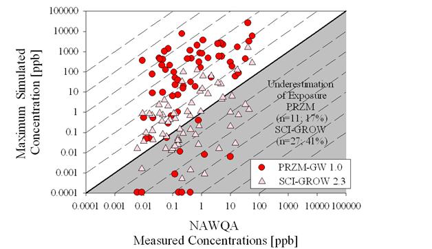
Figure A.1
Overlay of the PRZM-GW 1.0 and SCI-GROW 2.3 EDWCs compared to NAWQA monitoring data
In general, PRZM-GW provides conservative EDWCs compared to the monitoring data except for chemicals that are less mobile (i.e., Koc > 10,000). Although the SCI-GROW input parameter guidance indicates that this model should not be used for chemicals with Koc values > 9995 mL/goc, the SCI-GROW EDWCs for these chemicals is the result of the lower bound concentration limit (0.006 ppb per lb a.i./A applied) included in the SCI-GROW model. Thus, using SCI-GROW for these less mobile chemicals is a reasonable approach.
12 An overview of the NAWQA monitoring program is provided in the NAFTA Final Report1and is not repeated in this document.
13 Application rate and frequency were obtained from the most recent USEPA Drinking Water Exposure Assessment, which typically assesses the maximum application rate permitted by the registered label (consistent with USEPA/OPP policy).