US EPA - An Integrated Exposure and Effects Model for Probabilistic Risk Assessment (Aquatic level 2 Version 2x)
D. Randall*, K. Gallagher, J. Lin, D. Young, T. Barry, M. Echeverria, T. Bargar, D. Farrar, I. Kennedy, and I.M. Sunzenauer
*Office of Pesticide Programs, 1200 Pennsylvania Ave. N.W., Mail Code 7507C, Washington, DC 20460
telephone: 703-6051298
email: randall.donna@epa.gov
On this Page
- Introduction
- SAP Recommendations
- EPA's Refinements
- Initial Application Date
- Variable Volume Pond Model
- Distributions for Select Degradation Rates
- Generic Species Selection and Species Sensitivity Distribution
- Level 2 Version 2 Interface
- Errata
Introduction
For several years, the EPA's Office of Pesticide Programs (OPP) has been working towards a new tiered process for conducting ecological risk assessments for pesticides, to be used under the FIFRA regulatory framework. The new process includes incorporating measures of the probability and magnitude of potential effects in the second tier (Level 2). A pilot model for the preliminary probabilistic analyses was peer reviewed by the FIFRA Scientific Advisory Panel (SAP) and released to the public in March of 2001. Since that time, the Agency has been addressing the comments made during the peer review and has been refining the Level 2 model by developing a user-friendly, self-contained model for conducting preliminary probabilistic risk assessments. This eliminates the earlier model's need to use multiple external programs to conduct exposure and effects analyses. The newer model described here permits the user to easily conduct an exposure simulation, using an exposure module based on the Agency's PRZM 3.12 model (used here as a runoff model) and a variable volume pond (VVP) model. The exposure module has the capability to use distributions of selected input parameters and provides an output of predictions of pond concentrations and associated uncertainty. Inherent in the risk assessment model is also a toxicity data analysis module. The effects and exposure data are integrated using Monte Carlo and analytical solution methods in the probabilistic risk estimate module, yielding estimates of the probability and magnitude of risk to aquatic organisms, as well as estimates of uncertainty associated with those predictions. The results of analyses performed using this risk assessment model will be used by OPP's risk management divisions in decision-making.
SAP Recommendations
Among the recommendations made by the SAP concerning improvement of the pilot model were to:
Incorporate the ability to use distributions for selected exposure simulation model input parameters, potentially including parameters such as field size relative to pond size, metabolism rates, application dates, pH, curve number, and other potentially significant parameters.
Use the empirical data derived from the exposure simulation model in a bootstrapping approach to define the exposure distribution for a given distribution.
Incorporate a pond model that varies in size depending on inflow/outflow conditions.
EPA's Refinements
Since March 2001, the Agency has developed and incorporated the following refinements into the Level 2 refined aquatic risk assessment model for evaluating risk from land applied pesticides:
Exposure Analysis Module
Initial application date: Uses a range (uniform distribution) of possible initial application dates rather than a single initial application date.
Pond model: Incorporates a variable volume pond (VVP) model, which replaces EXAMS used previously.
Degradation rates: Allows choice of either deterministic or distribution- based input based on status of data availability (e.g., available metabolism rate data only meets the minimal data requirements versus existence of an enhanced data set).
Effects Analysis Module
Uses generic representative fish and invertebrate species (i.e., the 5th, 50th, and 95th percentiles of the respective species sensitivity distribution) rather than specific actual species.
Initial Application Date
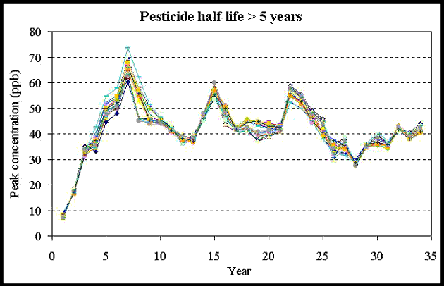
Incorporates initial application date as a uniform distribution rather than a single input date. This change was incorporated because of the sensitivity of the exposure output to selection of initial application day. The affect of changing initial application day, within a two week window, on annual peak pesticide concentrations in the model pond are explored in Figures 1a through 1c for three pesticides with different environmental half-lives, but using the same application rate, crop, soil and meterological data. In these examples, changing initial application date resulted in differences between the smallest and highest annual peak, for a given year, of 3.8 fold for the relatively non-persistent to moderately persistent pesticides and only about 1.4 fold for the persistent pesticide.
Figure 1.
Effect of Initial Application Day on Annual Peak Concentration for Three Pesticides:
Half-life
- <14 days
- 4 to 10 months
- >5 years
Figure 1a
Pesticide half-life < 14 days
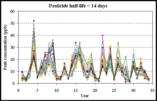
Figure 1b
Pesticide half-life 4 to 10 months
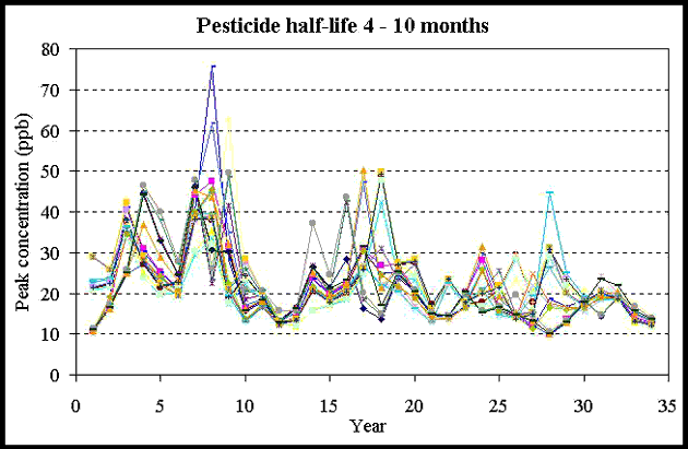
Figure 1c
Pesticide half-life > 5 years
Variable Volume Pond Model
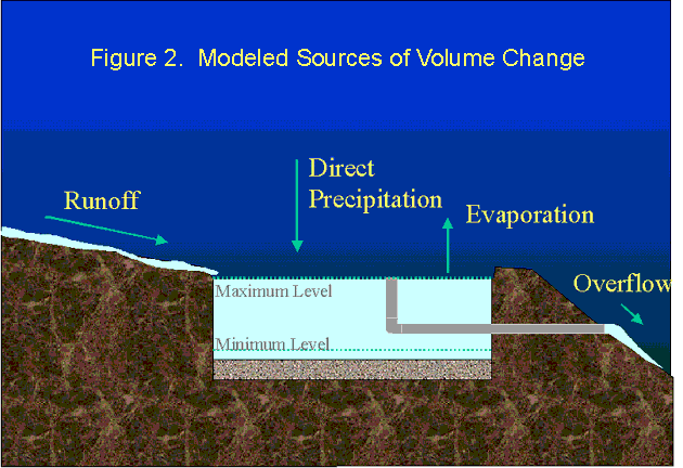
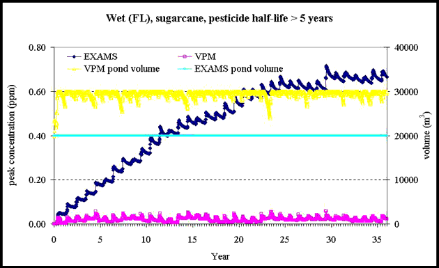
The Level 2 model incorporates a variable volume pond (VVP) model. Modeled sources of volume change incorporated in the VVP model are diagramatically presented in Figure 2. The affect of varying volume, as compared to the previous static pond model (EXAMS), was explored. Results for two pesticides, one relatively non-persistent the other persistent, under two very different climates are provided in Figures 3 and 4. Under arid conditions at a site in California the 2 m deep pond (i.e., standard pond evaluated in EXAMS) goes dry because there is insufficient precipitation and runoff to maintain water in the pond against evaporation. To allow evaluation the pond was not allowed to go dry, at least 1 cm depth was maintained at all times. As a result of evaporation, the volume in the pond was reduced resulting in higher concentrations than that predicted by the static 2 m pond (EXAMS). At a site in Florida, the reverse situation, consistent overflow occurs, and this despite an additional meter of storage added to the VVP. As a result of overflow pesticide mass leaves the pond resulting in lower concentrations than those predicted using EXAMS, which does not allow mass to leave the pond. In the particular situation chosen this difference was not large for the non-persistent, pesticide but it was very dramatic for the persistent pesticide. Appropriate settings for pond depth and runoff size in the VVP model are currently being evaluated for standard sites evaluated by OPP and will be incorporated into the Level 2 model. Other differences between the former exposure model (PRZM/ EXAMS) and PRZM/ VVP model are minor and are attributable to how temperature, photolysis, volatilization and peak identification are processed. The reason for these differences are listed in Table 1.
Figure 3
EXAMS versus VVP --Volume and Concentration (<4 day Half-life)
- Arid Clime
- Relatively Wet Clime
Figure 3a
Arid Clime
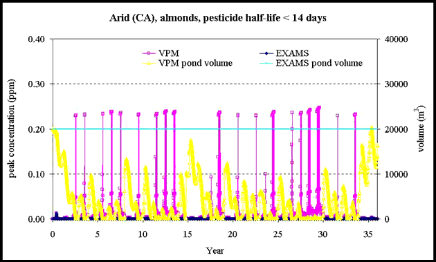
Figure 3b
Relatively Wet Clime
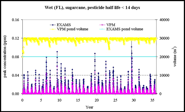
Figure 4
EXAMS versus VVP --Volume and Concentration (>5 year Half-life)
- Arid Clime
- Relatively Wet Clime
Figure 4a
Arid Clime
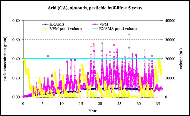
Figure 4b
Relatively Wet Clime
| PRZM/EXAMS | PRZM/VVP | |
|---|---|---|
| Soil deg. Rate* | Single precision | Double precision |
| Temperature | Calendar month | 30 day running mean |
| Photolysis | No reference latitude input (shell) | Reference lat. input |
| Volatilization | Const. wind speed | Daily wind speed |
| Peak identification | Calendar year | 365 day from application |
Distributions for Select Degradation Rates
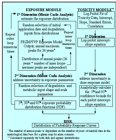
When there is sufficient data for such an approach, the exposure and risk analysis modules have been modified to incorporate the use of distributions of selected degradation and metabolic input parameters, such as Koc, soil aerobic half-life, aquatic aerobic half-life, benthic sediment half-life, photolysis, and hydrolysis. Because some pesticides may have only the minimal required fate data, which in most cases is insufficient for a distribution approach for input parameters, the Level 2 model has the option of generating the exposure distribution and characterizing uncertainty using point estimates for these input parameters. The use of point estimates for exposure input parameters is the same as that used in the pilot model. The current approach for determining the exposure distribution for minimal requirement fate data sets is outlined in Figure 5a and the approach for fate data sets that allow use of distributions for fate inputs is outlined in Figure 5b.
Figure 5
Approach Used for Calculation of Exposure and Probability-Response Curves
- Fate Inputs are Point Estimates
- Fate Inputs are Distributions
Figure 5a
Fate Inputs are Point Estimates
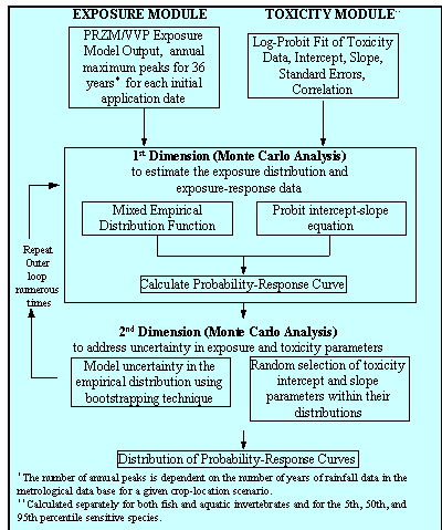
Figure 5b
Fate Inputs are Distributions
Generic Species Selection and Species Sensitivity Distribution
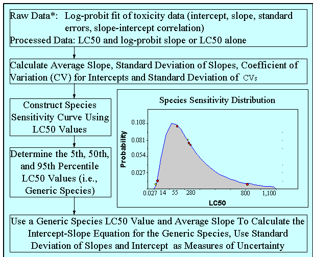
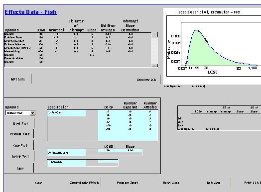
The toxicity or "effects" module has been designed to handle raw concentration-response data, and processed data that provides LC50 and log-probit slope or only LC50 values. For raw data a routine within the module determines if a log-probit model is appropriate and fits the data returning the slope, intercept, standard errors of the model, and the slope-intercept correlation. Once all the effects data have been entered, the LC50 data are used to construct a species sensitivity distribution. Separate analyses are conducted for fish and aquatic invertebrates. The current approach for determining the generic species and their concentration-response curves and measures of uncertainty are outlined in Figure 6.
Figure 6
Flowchart of Construction of Generic Species Concentration-Response Curve
Level 2 Version 2 Interface
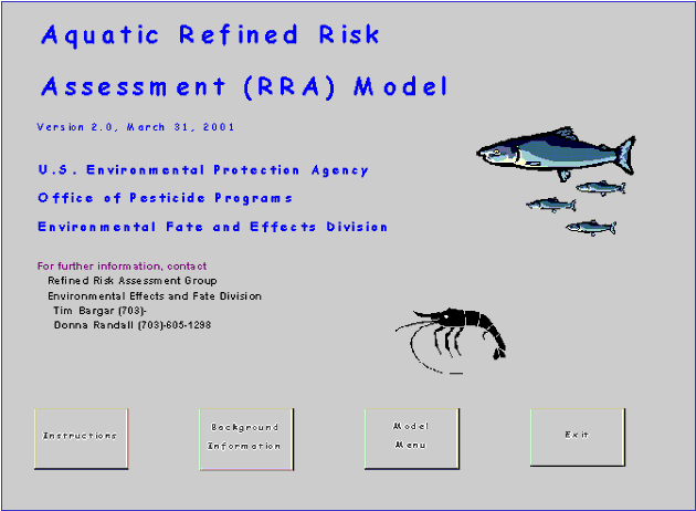
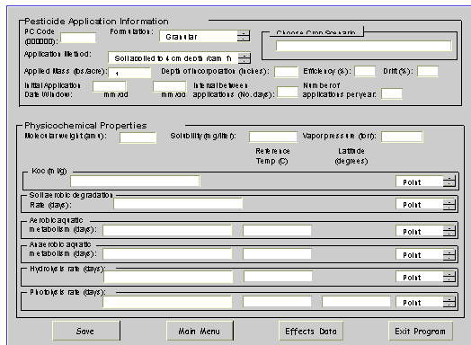
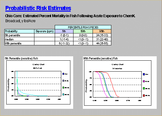
Current efforts for development of the Level 2 aquatic refined risk assessment model are focused on the creation of a user-friendly, integrated Level 2 model, which will incorporate exposure simulation modeling, toxicity test data analysis, and probabilistic simulation combining the exposure and effects data. The new model output will include tabular and graphical results. The goal of the integrated model is to facilitate more rapid and standardized analysis for Level 2 risk estimates. Some draft examples of user interfaces being created are provided below.
Peer review, beta testing, and implementation is currently scheduled for completion by fall 2003.
draft examples of user interfaces being created
Errata
In the second box of Figure 6, "...coffecient of variation (cv) for intercepts and standard deviation of cvs." should read "...mean relative standard error for intercepts and average standard error of slopes"
In the last box in Figure 6, "...use standard deviation of slope and intercept as measures..." be replaced with "use mean standard error of slopes and intercepts (scaled) as measures..."
![[logo] US EPA](../gif/logo_epaseal.gif)
