Ecological Committee on FIFRA Risk Assessment Methods (ECOFRAM)
Terrestrial Workgroup Report: V. Risk Characterization
On this Page
- Introduction
- Overview of Risk Assessment Methods
- Examples of Risk Assessment Methods
- Method 1: Point Estimate Quotients
- Method 2: Comparison of Exposure Distribution and Point Estimate for Effects
- Method 3: Comparison of Exposure and Effects Distributions
- Method 4: Distribution-Based Quotients
- Method 5: Integration of Exposure and Effects Distributions
- Levels of Refinement
- References
Introduction
Risk characterization is a final stage of ecological risk assessment where results of exposure and ecological effects analyses are integrated to evaluate the likelihood of adverse ecological effects occurring following exposure to a stressor. The ecological significance of the adverse effects should be discussed, including consideration of the types and magnitudes of the effects, their spatial and temporal patterns, and the likelihood of recovery (USEPA, 1992). This poster discusses methods for risk assessment for pesticides. Risk assessment is the analysis component of the risk characterization that integrates exposure and effects assessments to provide estimates of risk and evaluates uncertainties (USEPA, 1998). Risk estimates should be pertinent to the assessment endpoints that were defined in the Problem Formulation stage. The primary assessment endpoints determined by the ECOFRAM Terrestrial Workgroup were:
Effects on the survival and reproduction of individual birds and mammals.
Effects on population size and persistence of birds and mammals.
The risk characterization needs to place the output of the risk assessment in perspective and provide concise information that can be used for risk management. If the information is insufficient to support decisionmaking by risk managers, or the risk assessment needs to be further refined, it may be necessary to proceed to a further iteration of the risk assessment or to a higher level of refinement in the risk assessment process (see Levels of Refinement).
Overview of Risk Assessment Methods
A suite of risk assessment methods are recommended in order to provide the flexibility necessary to manage the diversity of pesticide scenarios for which a risk assessment is necessary (Fig. 1). Methods within the suite are grouped according to the level of sophistication, effort required, data required, and extent of refinement of the risk assessment. These methods can generally be divided into three categories:
Deterministic quotients
Comparison of exposure distribution to effects distribution (or fixed value)
Integration of exposure and effects distributions (Fig. 1; Methods 4, 5 and 6)
Examples of Risk Assessment Methods
Examples based on hypothetical data sets were developed to illustrate ecological risk assessment Methods 1 through 5. These examples are not case studies and do not provide a proof-of-concept but do allow a conceptual comparison of the methods and their risk assessment outputs. The examples use a single distribution of exposure values and three different sets of toxicity data, as follows:
The exposure data (mg/kg/d) to the left were fitted to a distribution below.
Distribution Type = Lognormal
Mean = 77.61
Standard Deviation = 40.05
95 percentile = 153.37
90 percentile = 128.56
| Exposure mg/kg/d | % Probability | % Cumulative |
|---|---|---|
| 30 | 10 | 10 |
| 33 | 10 | 20 |
| 45 | 10 | 30 |
| 60 | 10 | 40 |
| 81 | 10 | 50 |
| 88 | 10 | 60 |
| 89 | 10 | 70 |
| 95 | 10 | 80 |
| 120 | 10 | 90 |
| 126 | 10 | 100 |
Toxicity Data Sets
| LD50 mg/kg/d |
% Cum. |
|---|---|
| 150 | 20 |
| 155 | 40 |
| 195 | 60 |
| 210 | 80 |
| 350 | 100 |
| Parameter | Value |
|---|---|
| Distribution Type | Lognormal |
| Mean | 203.51 |
| Standard Deviation | 119.92 |
| 5 percentile | 71.43 |
| 10 percentile | 87.1 |
For each example, details of the output information on risk is provided to illustrate how the output could be interpreted. However, interpretation of the risk output is dependent on the exposure and effects inputs and what these represent. The explanation of risk is also dependent on the question being asked. The probabilistic risk assessment examples were generated using Crystal Ball, an EXCEL add-in for conducting model simulations. Using this software (and similar software e.g, @Risk) it is very easy to view data and to fit distributions to data. Distributions can be use to instead of a fixed value to represent the uncertainty around this value. Where actual data are available, these data should be preferentially used and the appropriate distribution should be carefully fitted to data. Selection of distributions based on minimal data, or data that poorly fit the distribution, should be used with caution.
| ↑ ↑ ↑ Less Realistic Risk Assessment ↑ ↑ ↑ |
Method 1 Point Estimate Quotients (deterministic) Exposure: Point estimate of exposure (mg/kg b.w./ unit time) Effects: Point estimate of toxicity (e.g., NOEL, LD50) Output: A ratio of exposure/toxicity (relative to risk but risk is not quantified) |
Ratio of single values of exposure and effects |
|---|---|---|
| Method 2 Comparison of Exposure Distribution with Point Estimate for Effects Exposure: Distribution of exposure (mg/kg b.w./ unit time) Effects: Point estimate of toxicity (e.g., NOEL, LD50) Output: Probability of exposure exceeding the effect level |
Risk based on a comparison of exposure and effect distributions (Probability of Exceeding a Fixed Value) | |
| Method 3 Comparison of Exposure and Effects Distributions (degree of overlap) Exposure: Cumulative frequency distribution of exposure (mg/kg b.w./ unit time) Effects: Distribution of toxicity for i. various species or ii. single species (e.g., LD50) Output: Probability of certain effect occurring when a fixed exposure level is exceeded | ||
| ↓ ↓ ↓ More Realistic Risk Assessment ↓ ↓ ↓ |
Method 4 Distribution-Based Quotients (uses Monte Carlo Simulations) Exposure: Distribution of exposure (mg/kg b.w./ unit time) Effects: Distribution of toxicity for i. various species or ii. single species (e.g., LD50) Output: Probability distribution of quotients (probability that exposure exceeds toxicity) | Risk based an integration of exposure and effects distributions |
| Method 5 Integrated Exposure and Effects Distributions (uses Monte Carlo Simulations) Exposure: Distribution of exposure (mg/kg b.w./ unit time) Effects: Distribution of toxicity (dose response distribution) Output: Probability of certain magnitude of effect (mortality) occurring | ||
| Method 6 Mechanistic/Process models Stage/Age structured; Meta-population; Individual-based; Spatially explicit models |
Method 1: Point Estimate Quotients
In the FIFRA regulatory process to date, the quotient method has been used in risk assessment for pesticides. A quotient of single values for exposure and effects are calculated (exposure value/toxicity value) and if the quotient exceeds a trigger value (equal to or less than 1), an adverse effect is considered likely to occur. The quotient values do not quantify risk but provide results that are relative to risk. An example assessment using the point estimate quotients approach is as follows:
| Inputs for Exposure and Effects (Toxicity Data Set 1) |
Exposure mg/kg/d |
Effects mg/kg/d |
Quotient Value (Exposure/Effects) |
|---|---|---|---|
| Based on 95 and 5 %tile | 153 | 71.4 | 2.14 |
| Based on 90 and 10%tile | 128.6 | 87.1 | 1.48 |
| Based on worst case data points | 126 | 90 | 1.40 |
The exposure values exceed the LD50 values resulting in quotient values greater than 1. This assessment does not indicate that an effect is unlikely. It does indicate that a refined assessment is necessary to determine the risk. The assessment provides no information on
- the probability of an effect occurring or
- the size of the effect.
Method 2: Comparison of Exposure Distribution and Point Estimate for Effects
In terrestrial vertebrate risk assessment, data supporting exposure assessments are likely more readily available than toxicity data. Consequently, models and resulting distributions are more easily obtainable for characterizing exposure than toxic effects. In this method, a single distribution of exposure is generated and a point estimate of toxicity is selected. Risk is estimated based on the probability of the effect level occurring within the distribution of exposure. This method is applicable where a dose-response is not available and toxicity is represented by a NOEL. This method is also applicable to situations where a point estimate of exposure is available and a distribution of effects.
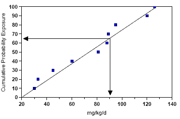
Fig. 2
Example of Method 2
(Comparison of Exposure Distribution with Point Estimate for Effects).
The point estimate for effects (90 mg/kg/day) has a 35% probability of being exceeded.
Method 3: Comparison of Exposure and Effects Distributions
Where sufficient data exists to provide meaningful distributions of both exposure and effects, these joint distributions can be compared to determine the extent of overlap. Risk can be expressed as a probability of exceedance of a fixed exposure level. Changes in the magnitude and likelihood of effects can be predicted for different exposure scenarios.
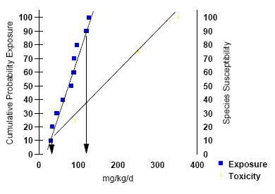
Fig. 3a
Example of Method 3
(Comparison of Exposure and Effects Distributions) using Toxicity Data Set 1. The y1 axis represents the % cumulative probability distribution for exposure and the y 2 axis represents the % species sensitivity or mortality.
Examples of Method 3
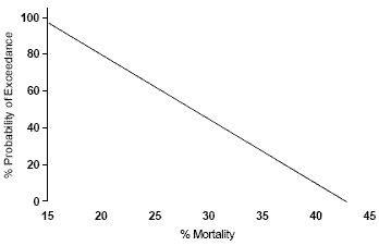
Fig. 3b
Example of Method 3
(Comparison of Exposure and Effects Distributions) using Toxicity Data Set 1 where % probability is represented as an exceedance for varying % mortality (or species sensitivity).
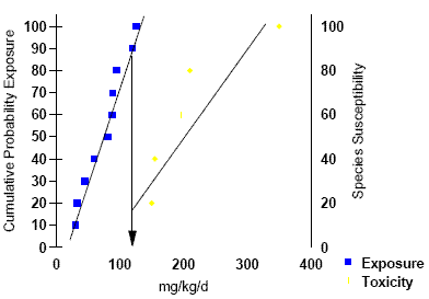
Fig. 4
Example of Method 3
(Comparison of Exposure and Effects Distributions) using Toxicity Data Set 2.
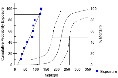
Fig. 5
Example of Method 3
(Comparison of Exposure and Effects Distributions) using Toxicity Data Set 3.
Method 4: Distribution-Based Quotients
In the Distribution-Based Quotient Method, each individual quotient represents a ratio of exposure to toxicity. The exposure and effects distributions are integrated using Monte Carlo simulations to sample values from distributions of exposure and toxicity to generate a probabilistic distribution of quotients. Risk is expressed from a probability distribution of quotient values, and the probability of the quotient exceeding 1 or any other quotient value. For example " There is a 20% probability that exposure levels exceed effect levels (based on a quotient of 1).
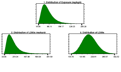
Fig. 6
Individual distributions of exposure
(graph 1) and toxicity (graphs 2 and 3).
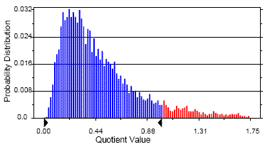
Fig. 7a
An example of ADistribution-based Quotients@ (Method 4) based on Toxicity Data Set 1 which contains multiple LD50 values. The right arrow shows a quotient value of 1.0 (equal to the 90th% tile).
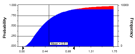
Fig. 7b
Distribution-based Quotients@ (Method 4) based on Toxicity Data Set 1 illustrated as a Cumulative Probability plot. The right arrow shows a quotient value of 1.0 (equal to the 90th%tile).
Method 5: Integration of Exposure and Effects Distributions
This method differs from Distribution-Based Quotients (Method 4) in that the quotient is replaced with a mortality response function so that the results of the risk assessment can be expressed as a probability of a certain magnitude of mortality (or some other effect). Three example models were developed. Assumptions of each example Model:
| Parameter | Model 1 | Model 2 | Model 3 |
|---|---|---|---|
| Dose (exposure) (D) | Lognormal Distribution | Lognormal Distribution | Lognormal Distribution |
| LD50 | Fixed Value | Normal Distribution | Normal Distribution |
| Slope | Fixed Value | Normal Distribution | Normal Distribution |
| Lab to Field Extrapolation Uncertainty Factor (UF) | none | None | UF= 75% Probability that the Field LD50 is within 2X Lab LD50 |
| N Individuals | 20 | 20 | 20 |
| N Simulations | 500 | 500 | 500 |
| Tolerance of each Individual (T) | T= LD50*10^(z/slope) z=standard normal distribution (x=0, σ =1) |
T= LD50*10^(z/slope) z=standard normal distribution (x=0, σ =1) |
T= (LD50*UF)*10^(z/slope) z=standard normal distribution (x=0, σ =1) |
| Fate of Each Individual | if D > T then mortality if D < T then survival |
if D > T then mortality if D < T then survival |
if D > T then mortality if D < T then survival |
The probability distributions shift to the right (the probability of mortality increases) as more uncertainty is considered in the model. This results from point estimates being replaced by distributions (Model 2 compared to Model 1) and uncertainty that was previously not explicit being quantified in the model (Model 3 compared to Model 2). The contribution of each source of uncertainty can be explored further in a sensitivity analysis.
The parameter assumptions in Models 1, 2 and 3.
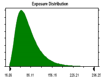
Exposure Distribution
Lognormal distribution with parameters:
5% - tile 31.02
95% - tile 153.37
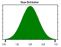
Slope Distribution
Normal distribution with parameters:
5% - tile 1.70
95% - tile 4.40
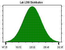
Lab LD50 Distribution
Normal distribution with parameters:
5% - tile 180.00
95% - tile 260.00
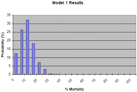
Model 1 Results
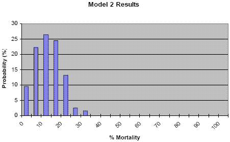
Model 2 Results
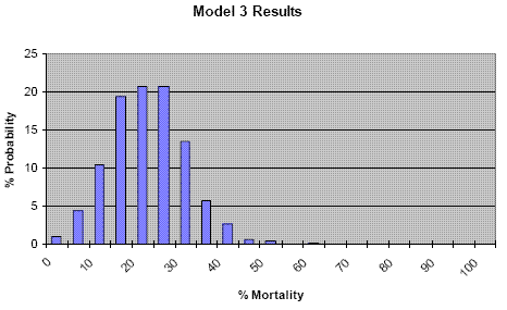
Model 3 Results
Levels of Refinement
The "Level of Refinement" refers to the extent that biological realism, risk and uncertainty are incorporated in the risk characterization and how well actual risk is described. In general the progression from lower to higher levels of refinement is based on:
Point estimates for parameters in the exposure assessment are replaced with distributions
Additional parameters in the exposure model are considered.
Increased spatial realism. Both treated and untreated habitats are considered
An improved estimate of mg/kg/b.w. per unit time for test animals
Number of species tested is increased
Pattern of exposure in toxicity test is refined
More uncertainty is explicitly considered in the analysis
Decreased uncertainty in the estimate of actual risk
Resource requirements will increase with level of refinement due to the development of additional data to support the probabilistic risk assessment and increased dependence on more complex models. Essentially the data allows parameters or factors used in the exposure or effects analysis that are unaccounted for in earlier levels (e.g., defaulted to 1) to be become explicit at higher levels of refinement. Parameters that are represented by point estimates may incorporate Probability Distribution Functions (PDFs) at higher levels of refinement. This concept is represented in Figure 11.

Figure 11
Parameter representation in analysis at different Levels of Refinement
Legend
 = parameter "off" or default to 1
 = parameter "on", represented by a point
 = parameter "on", represented by a PDF
| Level 1 | Level 2 | Level 3 | Sevel 4 | |
|---|---|---|---|---|
| Spatial | Treated Field PT=1 |
Treated Field & Nontarget areas PT < 1 |
Treated Field, Non-target areas & Drift Zone PT < 1 |
Landscape
|
| Unit Time | acute/ gorging = minutes, hours dietary = hours, days repro. = days |
acute/ gorging = minutes, hours dietary = hours, days repro. = days |
acute/ gorging = minutes, hours dietary = hours, days repro. = days |
acute/ gorging = minutes, hours dietary = hours, days repro. = days |
| Species of Concern | generic | generic focal |
focal | focal |
| Use Pattern | label maximum | label maximum |
|
|
| Crop | generic |
|
|
|
| Exposure Output |
|
|
|
|
| Effects Output |
|
|
|
Field options but only in combination with exposure assessments |
| Risk Characterization Method | Deterministic Quotients |
|
|
|
| Risk Characterization Output | Quotient | Probability distribution specific to method selected | Probability distribution specific to method selected | Probability distribution specific to method selected |
References
US Environmental Protection Agency, 1992. Framework for Ecological Risk Assessment. US Environmental Protection Agency, EPA/630/R-92/001.
US Environmental Protection Agency, 1998. Guidelines for Ecological Risk Assessment. US Environmental Protection Agency, EPA/630/R-95/002Fa.
![[logo] US EPA](../gif/logo_epaseal.gif)