Comments from Terrestrial Input Panel
Robert Luttik
Centre for Substances and Risk assessment of the National Institute of Public Health and the Environment in the Netherlands
On this Page
- Charge to ECOFRAM workshop panel members
- Is the draft report scientifically sound?
- Did the ECOFRAM Workgroup address the "charge" to the Terrestrial Workgroup?
- What are the limitations for predicting risk using the approach described in the draft report?
- What areas of the report need to be strengthened?
- At what point in the risk assessment process is the certainty level high enough to support the consideration of risk mitigation?
- Some general remarks
- Specific notes on the terrestrial draft
- Appendix on the derivation of extrapolation factors to predict a pre-determined protection level
Charge to ECOFRAM workshop panel members.
Is the draft report scientifically sound?
Yes I belief that the ECOFRAM Terrestrial draft report is the state of art of the moment.
I belief the ECOFRAM terrestrial draft report provides a basic framework for doing a probabilistic risk assessment. The report is providing a good review and description of recent developments in ecological risk.
Did the ECOFRAM Workgroup address the "charge" to the Terrestrial Workgroup?
Yes for birds they have certainly done the job, but for mammals and especially for reptiles a lot of research should be carried out to get those groups of animals to the same level as birds.
What are the limitations for predicting risk using the approach described in the draft report?
The moment you come to the third or fourth level of refinement much of the things you would like to know still have to be found out (lot of research is missing). I recognize that the higher levels of refinement can be used to pinpoint the research questions (as shown in the appendix C10 chlorpyrifos on apples), but in overall much research has to be carried for the higher levels of refinement.
Taking into account my answers to questions 1 to 3 the main areas of the report that need to be strengthened
are mammals and in particular the other terrestrial vertebrates and when this is not possible also recommendations should be given to close this gap.
Probably level two of refinement (tier 2) is the first level to consider risk mitigation
but this question is very difficult to answer and it depends to a large extend on the available information. When for instance the question is can we mitigate the risk of drift than the answer is probably yes because in this case the level of technical information and scientific understanding is enough to evaluate risk mitigation would be effective. But the moment animal behavior is coming into the picture the certainty level is probably not high enough.
Some general remarks
Take out the duplications.
Try to harmonize the two drafts (definitions and approaches, see also note on small sample problem) and perhaps an example as provided in Appendix C10 should also be included in the Aquatic report.
Specific notes on the terrestrial draft
First I would like to present/discuss some work done by two co-workers and myself several years ago . This work was published in 1996 by Traas, Luttik and Jongbloed in Ecotoxicology and Environmental Safety 34, 264-278 and the title is: A probabilistic model for deriving soil quality criteria based on secondary poisoning of top predators.
In this model we were particularly interested in factors that were important for the extrapolation of the laboratory to the field. These factors were:
- Caloric content,
- Food assimilation efficiency,
- Metabolic rate,
- Pollutant assimilation efficiency, and
- Species sensitivity
Some data on the caloric content (in kJ/g WW) and the water content of several food types are presented in Table 1. In this table I would like the reader to notice the low caloric content of leaves. In Table 2 the assimilation efficiency of several types of food birds are presented. And in this table I would like to point to the low assimilation efficiency of birds when eating leaves. It is also obvious that parameters like these can be used in probabilistic risk assessment. For the other three lab to field factors no probabilistic approach was recommended for the metabolic rate a factor of 2.5 was used for lab to field under normal circumstances and a factor of 4 in case of worst case scenario is used for more energy demanding periods.
Due to limited and contradictory information it was decided not to correct for pollutant assimilation efficiency and no special factor was used for the in literature mentioned differences between lab species and species in the field.
The first reason for presenting these data is that at page 2-20 it is proposed to use the following generic species:
- Small granivorous passerine birds or small mammals,
- Small insectivorous passerine birds or small mammals and
- Bird of prey that consumes small passerine birds and/or small mammals.
I would like to add a large grass consuming bird like a goose because of the low metabolic content of the food and the low food assimilation efficiency of these birds.
Related to this I would like to question the gorging scenario of the Canada goose and diazinon on Page C2-6. Perhaps there is another explanation. The combination of low caloric content of grass and the low food assimilation efficiency of grass eaters. In other words they just have to eat a lot of grass and are therefor more exposed.
The second reason is related to page 3-1. My question to the workgroup is: do you have considered using mg a.i. per kJ per day instead of mg a.i. per kg body weight per day. Nagy does give the relations between body weight and the caloric need. With using data based on the caloric content some of the problems of extrapolating from the lab to field would be solved.
Page 3-33 line 22 - 25 Avoidance (AV) versus Attraction
The opposite of avoidance is also occurring. Kononen et al. (ETC 5: 823-830 (1986) and ETC 6: 41-50 (1987)) measured the food consumption at each day of the food avoidance tests with methiocarb and carbofuran. The mallards exhibited definite avoidance behavior on day 1. Bobwhite demonstrated no or little avoidance behavior on the first day, avoidance occurred on the second day. In many of the examples they actually consumed more treated food than clean food.
As far as I would say AV could be larger than 1 but the draft only considers values between 0 and 1.
Page C2-5 (figure C2-1) avoidance AV figure
I do not think this figure is representing a normal case. In this figure the line for the reduction in consumption is going through the origin (zero is zero). I think that it is more reasonable that there is somewhere a threshold value, above a certain concentration the reduction will start.
Page 4-74 line 21
It is proposed that, until further work is done with the LC50 test, that the "extrapolation" factors developed with the LD50 be applied to the results of LC50 tests. I have the feeling that you should do this only for compounds, which do not have, or only slightly repellent properties.
Page C3-21 Grit size preference
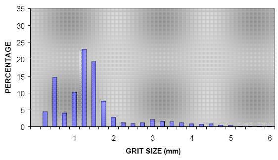
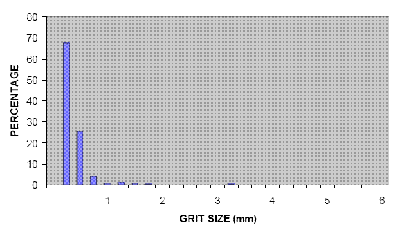
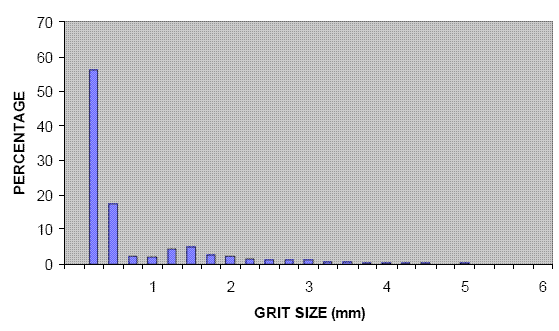
As stated at line 9-12 the grit size distribution profiles of most species have definite peaks, with the grit found in the gizzards declining abruptly on either side of the modal grit size. (line 9-12)
I do have my doubts about this generalization. I believe that there are two main categories of birds and one in between.
One group that is described by Best and Gionfriddo (birds that select a certain size of soil particles, see figure 1).
One group that does not select soil particles but that consumes soil particles just because they eat in that area (e.g. sticking to the food, see figure 2).
And a group that does both (selecting and unintentionally consuming, see figure 3).
| Food type | Caloric content | std. | n | %H2O |
|---|---|---|---|---|
| Fodder birds | 13.7 | 2.8 | 6 | 11 |
| Leaves | 0.9 | 0.7 | 7 | 92 |
| Seeds | 19.9 | 6.3 | 4 | 10 |
| Insect larvae | 5.2 | 3.3 | 8 | 77 |
| Insects adults | 7.2 | 1.6 | 10 | 66 |
| Birds | 7.9 | 2.1 | 49 | 66 |
| Mammals | 7.1 | 1.1 | 19 | 71 |
| Fish | 6.2 | 1.9 | 58 | 75 |
| Crustaceans | 4.4 | 1.4 | 12 | 67 |
| Food type | Assimilation efficiency | std | n |
|---|---|---|---|
| Bird fodder | 0.73 | 0.096 | 41 |
| Leaves | 0.37 | 0.075 | 6 |
| Seeds | 0.76 | 0.13 | 13 |
| Birds | 0.75 | 0.068 | 8 |
| Mammals | 0.75 | 0.072 | 39 |
| Fish | 0.78 | 0.04 | 15 |
| Insects larvae | 0.78 | 0.053 | 8 |
Figure 1 Size distribution of soil particles found in the gizzards of seedeaters

Figure 2 Size distribution of soil particles found in non-seedeaters

Figure 3 Omnivores but partly seed eaters

Appendix on the derivation of extrapolation factors to predict a pre-determined protection level
In chapter 3.5.3 methods are described for deriving extrapolation factors for birds (methods for mammals are also available (Luttik and Aldenberg 1995)). Very recently extrapolation factors were calculated for the aquatic ecosystem as well for single taxonomic groups (algae, crustaceans, fish and insects) as for the whole ecosystem. Values were derived for acute circumstances and chronic ones. The data presented in this appendix are preliminary data and are based on salt and freshwater species. Data for freshwater species will also be available in the near future.
Because not in all cases the log standard deviation is independent from the log mean the method described by Luttik and Aldenberg had to be extended.
In Table 3 the correlation coefficients, P-values, number of compounds on which the relation is based and the mean log standard deviation are presented. When the P-values are greater than 0.05 it is assumed that the standard deviation is independent from the mean (bold ones in Table) and for these groups it is possible to give fixed extrapolation factors for every sample size (n, see Table 4)
| Circumstance Type | Group of organisms | Correlation Coefficient | P-value | n | mean log std. |
|---|---|---|---|---|---|
| Acute toxicity E(L)C50 | Algae | -0.098 | 0.494 | 51 | 0.608 |
| Crustaceans | -0.336 | 0.000035 | 146 | 0.930 | |
| Fish | -0.206 | 0.00011 | 347 | 0.570 | |
| Insects | -0.356 | 0.0065 | 23 | 0.784 | |
| Aquatic ecosystem | -0.331 | 0.0000034 | 189 | 1.005 | |
| Chronic toxicity NOEC | Algae | +0.175 | 0.473 | 19 | 0.764 |
| Aquatic ecosystem | -0.55 | 0.67 | 62 | 1.128 |
For those other groups where the standard deviation is related to the mean first the unknown mean standard deviation has to be calculated by using the following relationships:
| Organism | Relationship |
|---|---|
| Crustaceans | y = -0.0978x + 1.1847 |
| Fish | y = -0.0518x + 0.7488 |
| Insects | y = -0.0984x + 0.9629 |
| Aquatic ecosystem | y = -0.0502x + 0.8747 |
Where y is the log standard deviation and x is the log mean.
And than the extrapolation factors can be calculated according to the following formulas:
SF50 = exp(162 * σ), and
SF95 = exp[1.62 + (1.64/vn)σ]
| n | Algae (acute) | Algae (chronic) | Aquatic ecosystem (chronic) | |||
|---|---|---|---|---|---|---|
| SF50 | SF95 | SF50 | SF95 | SF50 | SF95 | |
| 1 | 2.7 | 7.3 | 3.4 | 12.1 | 6.2 | 39.5 |
| 2 | 2.7 | 4.4 | 3.4 | 6.4 | 6.2 | 15.7 |
| 3 | 2.7 | 3.7 | 3.4 | 5.2 | 6.2 | 11.5 |
| 4 | 2.7 | 3.4 | 3.4 | 4.7 | 6.2 | 9.9 |
| 5 | 2.7 | 3.3 | 3.4 | 4.4 | 6.2 | 9.0 |
| 6 | 2.7 | 3.2 | 3.4 | 4.2 | 6.2 | 8.5 |
| 7 | 2.7 | 3.1 | 3.4 | 4.1 | 6.2 | 8.1 |
| 8 | 2.7 | 3.0 | 3.4 | 4.0 | 6.2 | 7.8 |
| 9 | 2.7 | 3.0 | 3.4 | 4.0 | 6.2 | 7.6 |
| 10 | 2.7 | 3.0 | 3.4 | 3.9 | 6.2 | 7.5 |
P.S. How to use these values? E.g. when only one chronic value for the aquatic ecosystemis available, this value should be divided by a factor of 39.5 to achieve the value that can be used in the risk assessment. When two chronic data are available for the aquatic ecosystem the geometric mean should be divided by a factor of 15.7.
![[logo] US EPA](../gif/logo_epaseal.gif)