An Integrated Exposure and Effects Model for Probabilistic Risk Assessment for Estimating Risks to Aquatic Organisms from Pesticides
K. Gallagher, J. Lin, D. Randall, D. Young, D. Farrar, T. Barry, Ian Kennedy, T. Bargar, L.W. Burns, I.M. Sunzenaeur
On this Page
- Introduction
- Revising the Ecological Assessment Process in USEPA Office of Pesticide Programs (OPP)
- Objectives of Refined Ecological Assessment Approach
- Four Levels of Refinement
- Background: Current Deterministic Level 1 Process
- New Level I: Refined Deterministic Screen
- Integrated Exposure and Effects Model for a Level 2 Probabilistic Assessment for Aquatic Organisms
- Aquatic Conceptual Model Flow Diagram
- New Additions to Water Body
- Variable Volume Water Body
- Draft Revised Level 2 Model Cover Page
- Model Background
- User Directions
- Exposure Module (Excerpt showing some input parameters)
- Effects Module (Data Entry Page)
- Species Sensitivity Distribution
- Model Output Example
- Work In Progress
Introduction
Introduction
Revising the Ecological Assessment Process in USEPA Office of Pesticide Programs (OPP)
1996: Case Study Risk Assessments to SAP- Recommended move towards PRA
1999: ECOFRAM Probabilistic Report drafts submitted and reviewed
2000: OPP presents general approach to Scientific Advisory Panel
2001: OPP presents case study of methods and Pilot Probabilistic Models to Scientific Advisory Panel
2002: OPP works toward finalizing more advanced, integrated, user friendly Level 2 probabilistic model
Objectives of Refined Ecological Assessment Approach
More closely reflect actual use scenarios and field conditions in higher tiered assessments
Build upon existing data requirements
Focus additional requirements on reducing key areas of uncertainty
Identify candidates for mitigation early in the process
Four Levels of Refinement
Level I - Refined Deterministic Screen
Level II - Preliminary Probabilistic Assessment
Level III - Refined Probabilistic Assessment
Level IV - Most Refined Probabilistic Assessment
Background: Current Deterministic Level 1 Process
Uses an index (risk quotient) of point estimates:
exposure estimates / toxicity endpointProvides a screen to identify pesticides not likely to pose an ecological risk
Supported by the FIFRA Scientific Advisory Panel (SAP) as a screening tool
Cannot address many risk management questions
e.g., Probability and magnitude of effects, population level impacts, etc.
New Level I: Refined Deterministic Screen
Similar to current deterministic assessment
Uses current exposure models and toxicity data requirements with some additions and modifications
Uses extrapolation factors to estimate species sensitivity differences
Conservative screen
Would distinguish low risk pesticides from potentially high risk pesticides
Integrated Exposure and Effects Model for a Level 2 Probabilistic Assessment for Aquatic Organisms
Consists of Three Modules:
Effects Module: Uses the FULL concentration-response curves
Exposure Module: Use the FULL range of the selected exposure distribution
Selected model input parameters can be entered as distributions
Effects and Exposure analyses are combined yielding predictions of likelihood and magnitude of effect
Aquatic Conceptual Model Flow Diagram
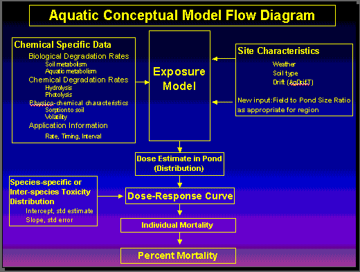
Aquatic Conceptual Model Flow Diagram
New Additions to Water Body
Variable volume water body
Parameters can change on daily basis (e.g., temperature, wind speed, dissipation rates)
Daily weather data from met files
Solved analytically (constant volume) or numerically (variable volume)
Variable Volume Water Body
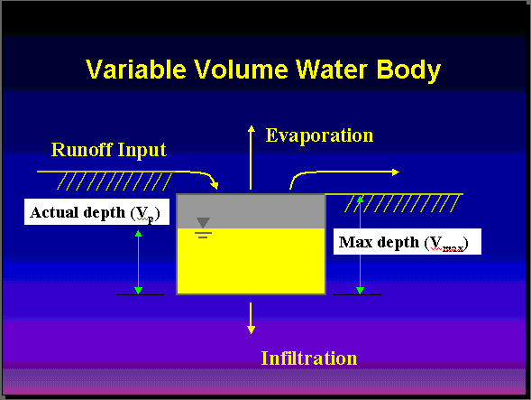
Variable Volume Water Body
Draft Revised Level 2 Model Cover Page
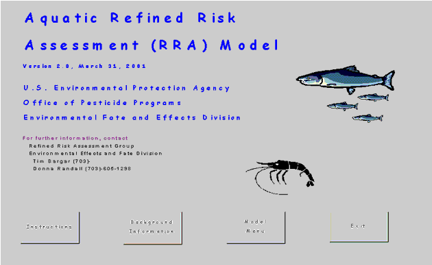
Draft Revised Level 2 Model Cover Page
Model Background
Background for the Aquatic RRA Model (Version 2.0)
The RRA Model estimates the joint probability acute risk function for an exposed aquatic population (i.e., determines the distribution of individual acute risks, based on the distribution of exposure data and distribution of toxic effects data) and the statistical uncertainty in the estimate of the joint probability function. This is accomplished using a 2-dimensional (2D) Monte Carlo Analysis program written in C by Timothy Barry for the Pilot Aquatic Risk Model, Version 1.0, and translated to MatLab. The basic exposure algorithm is
exposure = Inverse CDF (probability | parameters)
where probability is uniformly distributed, probability ∼ U(0,1), and parameters are the parameters of the fitted dose distribution. Inversion of the dose (or concentration) distribution is used to accommodate several distributions. Given an estimate of exposure, the risk is then calculated using the log-probit dose-response function
risk = Normsdist(intercept+slope*log(exposure))
where Normsdist is the Excel workbook function for the normal cumulative distribution function and intercept and slope are the parameters of the log-probit dose-response function. In order to run this model, characterizations of the uncertainty in each of the distributional parameters of the exposure distribution and dose-response function are needed. These are generally developed from the statistical uncertainty in the parameter estimates (e.g., derived from maximum likelihood) or based on expert judgment.
User Directions
Instructions for Conducting a 2D Simulation
An attempt has been made to make this user interface "user friendly" and relatively self explanatory. To run the 2D simulation model you will need to enter scenario-specific application data (e.g., chemical, crop, application rate, and location), which is referenced as Exposure Scenario Data in this program, and species-specific acute effects data (i.e., Effects Data). The specific Exposure Scenario data and Effects Data required to run the 2D model are described in the appropriate steps given below. There are instances where default values can be used rather than empirical data and this is identified where available. The program has been written to clearly document in the output the Exposure Scenario Data and Effects Data that was used to perform the simulation.
You will need to enter a complete Exposure Scenario and Effects Data File for the RRA simulation to run. To start entering the data, return to the Main Menu and select Model Menu.
The Model Menu page provides options for entering Exposure Scenario and Effects Data for a new project or opening an existing file (*.txt) and editing it as needed.
Effects Input Data -- Your have three choices for the type of acute toxicity data required.
(i)
IN YELLOW CELLS ONLY, Enter Best Estimates and Standard Errors for Exposure and Dose-Response Parameters, as well as their correlations, based on calculations made externally.
NOTE: Do not adjust values in green cells; Crystal Ball selects these during simulation.
This model is based on fitted chemical exposure distributions; the parameters' best estimates, their standard errors and correlation are required. Exposure data are based on pesticide usage on specific agricultural crops. the dose-response parameters are based on a log-probit fit to toxicity test data. This spreadsheet assumes that the individual parameters are normally distributed, with the specified central tendency (best estimate) and dispersion (stardard error).
3. In the Crop numeric cell (C15), change the fitted exposure distribution type for the inversion needed
- Clear cell contents if fitted exposure distribution is different from previous run.
- Use function wizard. select excel or user defined function as needed for particular fit inversion.
- Click on cells for shape (D6) and scale (D7) parameters as appropriate to assign function. Probability = cell C14
Directions are also given in cell comment on 2D page.
Exposure Module (Excerpt showing some input parameters)
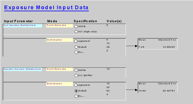
Exposure Module (Excerpt showing some input parameters)
Based on data available, user can input a 90th% value of a small data set, a multiple of an individual datum, or fit a distribution
Effects Module (Data Entry Page)
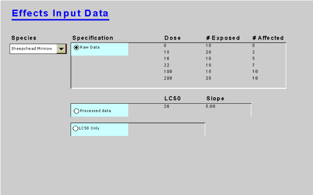
Effects Module (Data Entry Page)
Based on data available, user can evaluate raw toxicity test data,
use pre-analyzed data for LC50 and Slope, or use LC50 only
Species Sensitivity Distribution
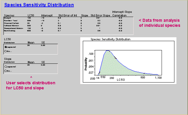
Species Sensitivity Distribution
Model Output Example
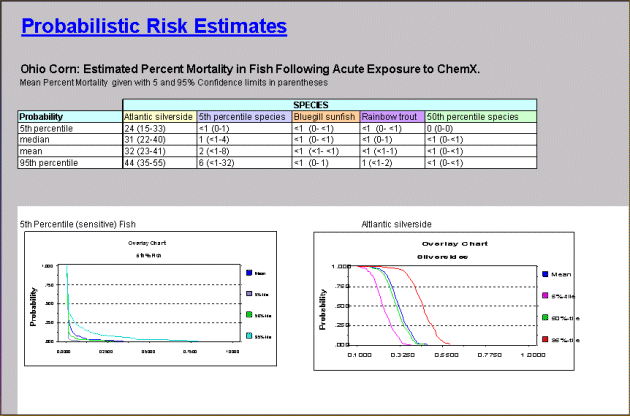
Model Output Example
Work In Progress
The model data entry template and exposure module and effects module are nearing completion
Work still needs to be done on output module: putting the data into a form that scientists and managers can readily use in their risk characterizations