Ecological Committee on FIFRA Risk Assessment Methods (ECOFRAM)
Terrestrial Workgroup Report: II. Exposure Assessment for Dietary Route

On this Page

Avian Exposure Pathways
Estimating exposure via contaminated food
Short-term and Long-term exposures
Levels of Refinement
Levels of Refinement in Dietary Exposure Analysis
Examples
- Biology Examples
- Chemistry Examples

Avian Exposure Pathways

Animals are exposed to pesticides through a variety of pathways. This poster focuses on exposure via contaminated food, but ECOFRAM is developing similar approaches for other pathways.

flow diagram with final target of total exposure in mg/kg/unit time from 3 sources: (1) inhalation that is also the target of source air, (2) dermal that is also the target of sources: direct contact, surface water, soil, and vegetation and (3) total oral which is also the target of two sources: (1) dietary(food) which is itself a target of sources: vertebrate prey, invertebrate prey, seeds and fruits, and vegetation, (2) other oral (non food) which is also the target of sources: granules/baits, preening, soil, and surface water.

Top of page

Estimating exposure via contaminated food

Exposure via contaminated food is estimated using the dietary dose equation, adapted from Pastorok et al. (1996).

DD = ∑ FIR · AV_Ci · PD_i · PT_i · C_i · FDR_i /W

Where:

DD = dietary dose (mg pesticide/kg body weight/unit time)

FIR = Food ingestion rate

AV_Ci = Avoidance factor at concentration C_i

PD_i = Proportion of food type i in the diet

PT_i = Proportion of food type i obtained in treated area

C_i = Concentration of pesticide in food type i

FDR_i = Fresh to dry weight ratio for food type i

W = Body weight

Top of page

Short-term and Long-term exposures

Exposure is estimated on two time scales:

short-term exposure - over a period of minutes to a few hours. This is proposed for assessing exposures due to gorge feeding, where animals consume much or even all of their daily intake of food in a very short period. Gorging behavior may only occur in special circumstances, when food is freely available and the pressure to feed is high. This type of exposure should be assessed by comparison with acute oral toxicity.
long-term exposure - over periods of hours to days or weeks. This is the more usual scenario, where food is consumed gradually over time. This type of exposure should be assessed by comparison with acute dietary toxicity or reproductive toxicity.

Top of page

Levels of Refinement

Each input to the dietary dose equation may be estimated at up to 4 different levels of refinement, as shown in the following Tables. Exposure by other pathways may be treated in similar ways.

Level I is intended as a simple Screening Level Assessment. It produces a point estimate and is based on "reasonable worst case" assumptions for each input parameter. Its purpose is to assist the assessor in deciding whether the dietary route is significant enough to warrant more detailed analysis at Levels II-IV.

Top of page

	Level 1	Level 2	Level 3	Level 4
PURPOSE	Produce point estimate of reasonable worst case dietary exposure for generic species Short- and long-term exposure estimated separately	Estimate distribution of exposures for focal species Use simple estimates of distributions for input variables, based on existing data or expert judgement Separate short- and long-term estimates	As Level 2 but use more refined estimates of input distributions Also, take account of exposure due to spray drift	More refined assessment which may include: field studies to estimate input distributions in relevant conditions distributions based on explicit landscape models

Biology inputs

Biology inputs
Parameter	Level 1	Level 2	Level 3	Level 4
FIR - food intake rate (dry weight)	Use existing estimates of intake, e.g. Nagy's equations Adjust to reasonable worst case (e.g. 3 x average daily intake) For long-term exposure, assume feeding rate constant over time	Hypothetical distribution (e.g. Triangular, from 33% to 300% of average), or Normal distribution based on confidence intervals Allow food intake to vary over time Assess relative frequency of gorging behavior	Obtain raw data underlying average FIR and use to estimate distribution	Field data on actual FIR in relevant conditions
PD_i - proportion of diet from each food type	Reasonable worst case - assume diet consists entirely of the food type with the highest residues	Hypothetical distributions based on published data	Obtain raw data underlying published values and use to estimate distributions	Field data on actual PD in relevant conditions
PT - proportion of food from treated area	Reasonable worst case - PT=1 (100% of food obtained from treated area)	Allow PT < 1, i.e. take account of untreated area. Use existing information and expert judgment to estimate distribution of PT	As for Level 2 but also take account of time spent in drift zone and residue levels there	Field data on actual PT in relevant conditions Landscape models using GIS to overlay animal movements on residue distributions
AV_Ci - avoidance	Reasonable worst case - AV_Ci = 1 (animal does not avoid contaminated food)	Estimate AV_Ci from food consumption in dietary toxicity tests to decide whether avoidance may be important in short- and long-term exposures.	Conduct special studies to estimate AV_Ci for typical and worst- case conditions Separate studies required for short- and long-term scenarios	More complex studies with captive animals to quantify the distribution of AV _Ci under the range of relevant conditions
FDR_i - Fresh to dry weight ratio.	Use average estimates for relevant food types, from the literature	Use confidence limits for these estimates to define hypothetical distributions	Obtain raw data underlying published values and use to estimate distributions	Field data on actual FDR in relevant conditions Consider dessication of food items
W, body weight	Use average estimates for relevant species, from the literature	Hypothetical distributions around published means Allow for age/sex differences	Obtain raw data underlying published values and use to estimate distributions	Field data on actual W in relevant conditions

Chemistry inputs

Chemistry inputs
Parameter	Level 1	Level 2	Level 3
RESIDUES IN FOLIAGE - seeds, fruits, grasses etc.	Distribution of initial residues estimated from application rate using empirical relationship (Fletcher et al.) Dissipation over time - use distribution from Willis database, or estimate from soil degradation rate	Model (under development)	Field studies for validation and/or calibration of models
RESIDUES IN INVERTEBRATES - insects, earthworms etc.	Distribution of initial residues estimated from application rate using empirical relationship (under development) Dissipation over time - use existing distributions if available	Model (requires development - difficult due to variation in exposure of invertebrates)	Field studies for validation and/or calibration of models
RESIDUES IN VERTEBRATES - small birds and mammals, amphibians etc.	Estimate exposure of vertebrates through their food over time (see above) Estimate depuration rates using data from chickens or rats (one compartment model) Compute resulting body burdens and use as estimates of dose to predators	As Level 1 but more sophisticated model with more compartments (requires development)	Field studies for validation and/or calibration of models

Analysis outputs

Analysis outputs
Level 1	Level 2	Level 3	Level 4
Short-term exposure Reasonable worst case dose for single gorging bout, mg/kg body weight	Short-term exposure Distribution of doses for single gorging bout, mg/kg body weight Approximate estimate of frequency of gorging behavior (e.g. gorging bouts per individual per day), and/or identification of conditions under which gorging may occur (e.g. flock feeding, abundant food source)	Short-term and Longterm As for Level 2 but: distributions for more input parameters, based on better data improved estimates of the frequency of gorging behavior consideration of drift zone in Long-term assessment.	Short-term and Longterm As for Level 3 but: distributions based on explicit spatial models field studies conducted to estimate distributions for focal species in relevant conditions
Long-term exposure Dose in mg/kg/day for days 1, 2, 3 etc. (as required) after pesticide application Peak daily dose Time-weighted average dose over any relevant time period (e.g. 5 days, 21 days)	Long-term exposure Dose in mg/kg/hour, reflecting diurnal variation in feeding activity Distribution for each hour on days 1, 2, 3 etc. After pesticide application Distributions for peak hourly dose and peak daily dose Distribution of time-weighted averages over any period

Top of page

Examples

Biology Examples

PT - Proportion of time in treated area - Level 4

Crocker et al.. (in prep.) measured PT for European blackbirds in UK apple orchards by radio-tracking. Most individuals spent less than 10% of their time in the central (i.e. sprayed) area of the orchard, but a few individuals spent up to 70% of their time there. This provides a distribution of PT which could be used in a Level 4 exposure analysis.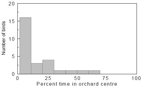

AV_Ci - Avoidance of treated food - Level 2

To assess whether animals may limit their exposure by avoiding treated food, AVCi may be estimated from the avian dietary toxicity test. Points represent consumption of fonofos-treated diet on first day of test, expressed as a proportion of consumption by control groups fed untreated diet (data from Hill and Camardese, 1986).
C_i = concentration in test diet, ppm.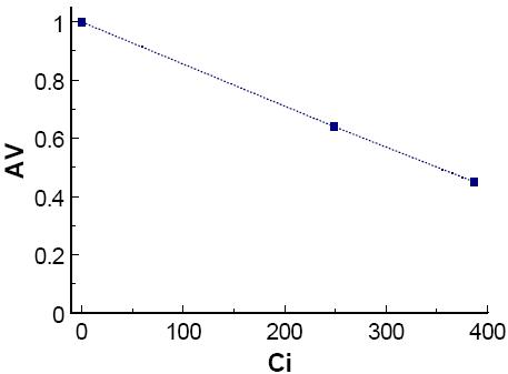
Chemistry Examples

RESIDUES IN FOLIAGE - Level 1
- A simple model allowing for multiple applications and first order dissipation of the residues:
  
  Equation (1)
  
  C_f (t=t_N) = _i=1∑^N (m_i / M _f) exp[-k (t_N - t_i)]
  
  Where:
  
  C_f (t=t_N) = foliar concentration immediately after the Nth application in chemical mass/foliar mass
  
  m_I = chemical mass applied to foliage during application i (mg)
  
  M_f = foliar mass (kg)
  
  K = overall first order foliar dissipation rate constant (1/day)
  
  t_N = time of Nth application (day)
  
  t_I = time of ith application (day)
- The concentration at any time t' after the Nth application is given by:
  
  Equation (2)
  
  C_f (t=t') = C_N exp[-k (t' - t_N)]
- The ratio m_i / M_f for each application i in equation (1) can be estimated probabilistically for various food types from the distributions of field measurement data reported by Fletcher et al:
  
  Equation (3)
  
  (m_i / M_p) = (Fletcher value normalized to 1 lb ai/acre) * (application rate in lbs ai/acre)
RESIDUES IN FOLIAGE - Level 2

Computer models take into account additional factors that affect foliar concentrations such as plant growth, uptake by plants, and wash-off from plants. Based upon mass-balance considerations, computer models first generate an equation relating the total rate of change in foliar concentration to the sum of changes due to individual processes that affect the concentration:

Equation (4)

(dC_f / dt)_total = (dC_f / dt)_app + (dC_f / dt)_uptake - (dC_f / dt)_growth - (dC_f / dt)_dissipation - (dC_f / dt)_wash-off

Equation (4) is then solved to give the foliar concentration as a function of time, C_f(t). This can provide peak concentrations and average concentrations over any desired time period. The output can also be graphically presented as plots of C_f versus time.

At both Levels, the analysis may be either deterministic or probabilistic. In probabilistic modeling, one or more of the inputs are distributions. This produces a distribution of estimates of the foliar concentration for each time step.